Assessing the effect of random missing data
Robert W Schlegel
2018-09-05
missing_data.RmdOverview
The purpose of this vignette is to quantify the effects that missing data have on the detection of events. Specifically, the relationship between the percentage of missing data, as well as the consecutive number of missing days, on how much the seasonal climatology, the 90th percentile threshold, and the MHW metrics may differ from those detected against the same time series with no missing data.
The missing data will be ‘created’ by striking out existing data from the three pre-packaged time series in the __heatwaveR__ package, which themselves have no missing data. This will be done in two ways:
- the first method will be to simply use a random selection algorithm to indiscriminately remove an increasing proportion of the data;
- the second method will be to systematically remove data from specific days/times of the year to simulate missing data that users may encounter in a real-world scenario
- one method will be to remove only weekend days from the data
- another method is to remove only winter data to simulate ice-cover
It is hypothesised that the more consecutive missing days of data there are, the bigger the effect will be on the results. It is also hypothesised that consecutive missing days will have a more pronounced effect/be a better indicator of time series strength than the simple proportion of missing data. A third hypothesis is that there will be a relatively clear threshold for consecutive missing days that will prevent accurate MHW detection.
library(tidyverse)
library(broom)
library(heatwaveR)
library(lubridate) # This is intentionally activated after data.table
library(fasttime)
library(ggpubr)
library(boot)
library(FNN)
library(mgcv)
library(padr)
# A clomp of functions used below
# Written out here for tidiness/convenience
# Quantify consecutive missing days
con_miss <- function(df){
ex1 <- rle(is.na(df$temp))
ind1 <- rep(seq_along(ex1$lengths), ex1$lengths)
s1 <- split(1:nrow(df), ind1)
res <- do.call(rbind,
lapply(s1[ex1$values == TRUE], function(x)
data.frame(index_start = min(x), index_end = max(x))
)) %>%
mutate(duration = index_end - index_start + 1) %>%
group_by(duration) %>%
summarise(count = n())
return(res)
}
# Function for knocking out data but maintaing the time series consistency
random_knockout <- function(df, prop){
res <- df %>%
# group_by(site) %>%
sample_frac(size = prop) %>%
# arrange(site, t) %>%
arrange(t) %>%
pad(interval = "day") %>%
full_join(sst_cap, by = c("t", "temp", "site")) %>%
mutate(miss = as.character(1-prop))
return(res)
}
# Calculate only events
detect_event_event <- function(df, y = temp){
ts_y <- eval(substitute(y), df)
df$temp <- ts_y
res <- detect_event(df)$event
return(res)
}
# Run an ANOVA on each metric of the combined event results and get the p-value
event_aov_p <- function(df){
aov_models <- df[ , -grep("miss", names(df))] %>%
map(~ aov(.x ~ df$miss)) %>%
map_dfr(~ broom::tidy(.), .id = 'metric') %>%
mutate(p.value = round(p.value, 5)) %>%
filter(term != "Residuals") %>%
select(metric, p.value)
return(aov_models)
}
# Run an ANOVA on each metric of the combined event results and get CI
event_aov_CI <- function(df){
aov_models <- df[ , -grep("miss", names(df))] %>%
map(~ aov(.x ~ df$miss)) %>%
map_dfr(~ confint_tidy(., parm = ), .id = 'metric') %>%
mutate(miss = rep(c("0", "0.1", "0.24", "0.50"), nrow(.)/4)) %>%
select(metric, miss, everything())
return(aov_models)
}
# A particular summary output
event_output <- function(df){
res <- df %>%
group_by(miss) %>%
# select(-event_no) %>%
summarise_all(c("mean", "sd"))
return(res)
}Random missing data
Knocking out data
First up we begin with the random removal of increasing proportions of the data. We are going to use the full 33 year time series for these missing data experiments.
# First put all of the data together and create a site column
sst_ALL <- rbind(sst_Med, sst_NW_Atl, sst_WA) %>%
  mutate(site = rep(c("Med", "NW_Atl", "WA"), each = 12053))

# Create a data.frame with the first and last day of each time series
# to ensure that all time series are the same length
sst_cap <- sst_ALL %>%
  group_by(site) %>%
  filter(t == as.Date("1982-01-01") | t == as.Date("2014-12-31")) %>%
  ungroup()

# Now let's create a few data.frames with increased proportions of missing data
sst_ALL_miss <- sst_ALL %>%
  mutate(site2 = site) %>%
  nest(-site2) %>%
  mutate(prop_10 = map(data, random_knockout, prop = 0.9),
         prop_25 = map(data, random_knockout, prop = 0.75),
         prop_50 = map(data, random_knockout, prop = 0.5)) %>%
  select(-data) %>%
  gather(key = prop, value = output, -site2) %>%
  unnest() %>%
  select(-site, -prop) %>%
  rename(site = site2)
Consecutive missing days
With some data randomly removed, let’s see how consecutive these missing data are.
# And now the results
sst_ALL_con <- sst_ALL_miss %>%
  group_by(site, miss) %>%
  nest() %>%
  mutate(data2 = map(data, con_miss)) %>%
  select(-data) %>%
  unnest()

# Visualise
ggplot(sst_ALL_con, aes(x = as.factor(duration), y = count, fill = site)) +
  geom_bar(stat = "identity") +
  facet_grid(site~miss, scales = "free_x") +
  labs(x = "consecutive missing days")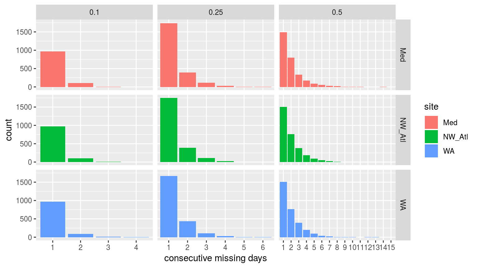
Bar plots showing the count of consecutive missing days of data per time series at the three different missing proportions.
It is reassuring to see that for the 10% and 25% missing data time series there are very few days of consecutive missing data greater than two. This is good because the default MHW detection algorithm setting is to interpolate over days with 2 or fewer missing values. It is therefore unlikely that 1 or 2 consecutive days of missing data will affect the resultant clims or MHWs.
Seasonal signal
sst_ALL_clim <- sst_ALL %>%
  mutate(miss = "0") %>%
  rbind(., sst_ALL_miss) %>%
  group_by(site, miss) %>%
  nest() %>%
  mutate(clim = map(data, ts2clm, climatologyPeriod = c("1982-01-01", "2014-12-31"))) %>%
  select(-data) %>%
  # gather(key = clim, value = output, -site) %>%
  unnest()

# Pull out only seas and thresh for eas of plotting
sst_ALL_clim_only <- sst_ALL_clim %>%
  select(site:doy, seas:var) %>%
  unique()

# visualise
ggplot(sst_ALL_clim_only, aes(y = seas, x = doy, colour = miss)) +
  geom_line(alpha = 0.3) +
  facet_wrap(~site, ncol = 1, scales = "free_y") +
  labs(x = "calendar day of year", y = "temp (C)")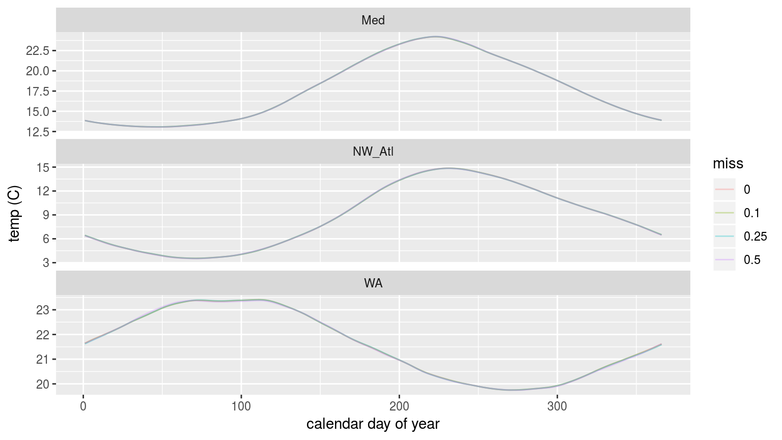
The seasonal signals created from time series with increasingly large proportions of missing data.
As we may see in the figure above, there is no perceptible difference in the seasonal signal created from time series with varying amounts of missing data.
90th percentile threshold
ggplot(sst_ALL_clim_only, aes(y = thresh, x = doy, colour = miss)) +
  geom_line(alpha = 0.3) +
  facet_wrap(~site, ncol = 1, scales = "free_y") +
  labs(x = "calendar day of year", y = "temp (C)")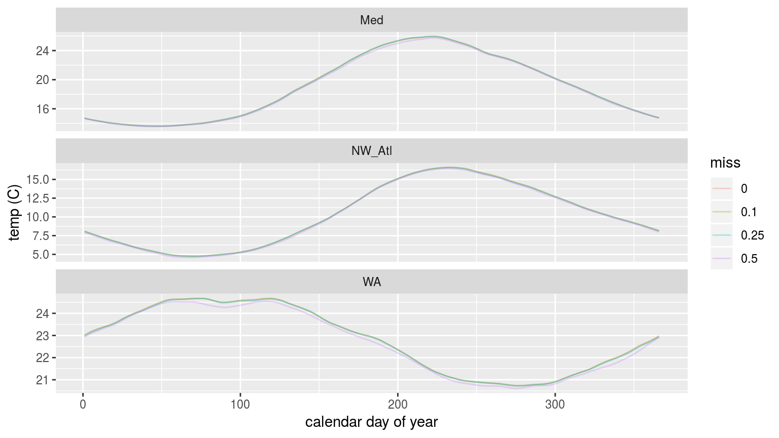
In the figure above we are able to see that the 90th percentile threshold is lower for the time series missing 50% of their data, but that 10% and 25% do not appear different. This is most pronounced for the Western Australia (WA) time series. This will likely have a significant impact on the size of the MHWs detected.
Before we calculate the MHW metrics, let’s look at the output of an ANOVA comparing the seasonal and threshold values against one another across the different proportions of missing data.
sst_ALL_clim_aov <- sst_ALL_clim %>%
  select(-t, - temp, -doy) %>%
  mutate(miss = as.factor(miss)) %>%
  unique() %>%
  group_by(site) %>%
  nest() %>%
  mutate(res = map(data, event_aov_p)) %>%
  select(-data) %>%
  unnest()

ggplot(sst_ALL_clim_aov, aes(x = site, y = metric)) +
  geom_tile(aes(fill = p.value)) +
  geom_text(aes(label = round(p.value, 2))) +
  scale_fill_gradient2(midpoint = 0.1)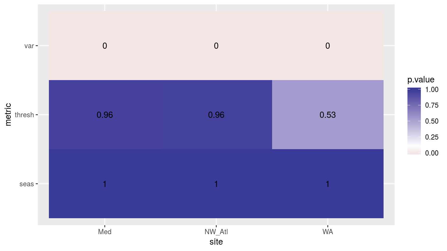
Heatmap showing the ANOVA results for the comparisons of the clim values for the four different proportions of missing data. Only the variance in the climatologies are significantly different at p < 0.05.
If one were to compare this heatmap to those generated by reducing time series length, one would see that the effect of shorter time series on discrepancy between the thresholds is much greater than for missing data.
MHW metrics
Now that we know that as much as 50% missing data from a time series does not produce significantly different thresholds, we now want to see what the downstream effects of these slight differences are on the MHW metrics.
# Calculate events
sst_ALL_event <- sst_ALL_clim %>%
  group_by(site, miss) %>%
  nest() %>%
  mutate(res = map(data, detect_event_event)) %>%
  select(-data) %>%
  unnest() #%>%
  # filter(date_start >= "2002-01-01", date_end <= "2011-12-31") %>%
  # select(-c(index_start:index_end, date_start:date_end))
# ANOVA p
sst_ALL_aov_p <- sst_ALL_event %>%
select(site, miss, duration, intensity_mean, intensity_max, intensity_cumulative) %>%
nest(-site) %>%
mutate(res = map(data, event_aov_p)) %>%
select(-data) %>%
unnest() #%>%
# spread(key = metric, value = p.value)
# visualise
ggplot(sst_ALL_aov_p, aes(x = site, y = metric)) +
geom_tile(aes(fill = p.value)) +
geom_text(aes(label = round(p.value, 2))) +
scale_fill_gradient2(midpoint = 0.1) +
theme(axis.text.y = element_text(angle = 90, hjust = 0.5))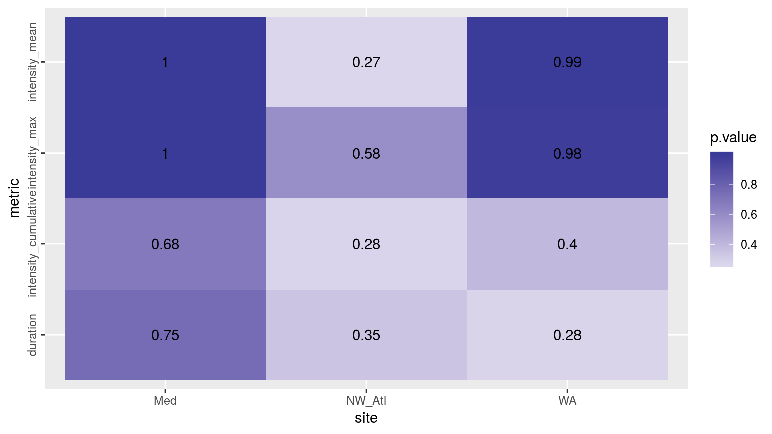
Heatmap showing the ANOVA results for the comparisons of the main four MHW metrics for the four different proportions of missing data. There are no significant differences.
As we may see in the figure above, there are no significant differences between the main MHW metrics depending on how much data are missing from a time series. The metrics differ most in the North West Atlantic (NW_Atl) time series, but are not significant.