Alternative climatologies and baselines
AJ Smit
2018-09-05
Climatologies_and_baselines.RmdBackground
A time series of temperatures taken at a specific locality is a sample of the thermal environment. Because it is a sample, which is used to approximate the true state of the environment, the representivity of the data is subject to certain limitations that have an influence on their accuracy and precision—in other words, on how well the data represent reality. Here we will not concern ourselves with matters of precision and accuracy; rather, we shall deal with ways to produce climatologies from a time series of daily thermal measurements.
A climatological mean is a multi-year average over a base period of typically 30 years duration. Sometimes the climatology is also called a ‘climate normal.’ It predicts the temperatures over an annual cycle that will most likely be experienced at a particular place and time.
Another concept that we use here instead of a climatology is a baseline…

Figure 1. Processing pipeline in the detect() algorithm with emphasis on the climatology and baseline procedures. The dark black arrows indicate the options that are currently available.
The default climatology and threshold
Central to the functioning of the heatwaveR detect algorithm is the climatology, which is the reference against which the extremes are calculated. For historical reasons—which also turn out to make good practical sense—it has become standard practice to base a climatology on 30 years’ worth of data, updated at the start of each new decade (the most recent being 1981-2010). For the heatwaveR package we recommend the same. Because heat wave detection is based on daily data, a daily climatology is required. That is, the mean value for each of the days in a 365 (non-leap) or 366 (leap) day long year. In the case of gridded data, we also require that the climatology is at the same spatial resolution as the SST time series within which the extreme events are sought. In the case of the dOISST v2. data, it is independently calculated at each of the 1/4° grid cells, and for station data it must be representative of that station and preferably also obtained with the same instrument that yielded the seawater temperature time series entering the event detection algorithm (in fact, the algorithm will by default use the daily time series to derive the climatology).
In a daily climatology, there will be one mean temperature for each day of the year (365 or 366 days, depending on how leap years are dealt with). How the daily mean is calculated can vary somewhat from application to application. The detect() function applies a window centred on a sliding Julian day for the pooling of values that will form the basis for calculation of the climatology and threshold percentile. We use a default of 5 days, which gives a window width of 11 days centred on the 6th day of the series of 11 days. For example, the mean temperature for Julian day 6 will be comprised of all temperatures measured from Julian days 1 to 11, across 30 years, i.e. 330 temperature measurements are summarised in this climatological daily mean. A sliding window centred on Julian day 7 will comprise all temperatures measured on Julian days 2 to 12 over the 30 years; etc. Currently we do not provide the option to calculate a weighted mean; rather, each day receives the same weighting as any other day, irrespective of how far the day is from the one on which the sliding window is centred. Climatologies produced with sliding windows of width 1, 11, 31, and 61 days are presented in Figure 1. In the figure we see that the wider the sliding window becomes the less day-to-day noise is retained in the climatology.
library(tidyverse) # misc. data processing conveniences
library(lubridate) # for working with dates
library(heatwaveR)
# Using a built-in data set
# smoothPercentile = FALSE
res.1.F <- ts2clm(sst_WA, climatologyPeriod = c("1983-01-01", "2012-12-31"),
windowHalfWidth = 0, smoothPercentile = F, clmOnly = TRUE)
res.11.F <- ts2clm(sst_WA, climatologyPeriod = c("1983-01-01", "2012-12-31"),
smoothPercentile = F, clmOnly = TRUE)
res.31.F <- ts2clm(sst_WA, climatologyPeriod = c("1983-01-01", "2012-12-31"),
windowHalfWidth = 15, smoothPercentile = F, clmOnly = TRUE)
res.61.F <- ts2clm(sst_WA, climatologyPeriod = c("1983-01-01", "2012-12-31"),
windowHalfWidth = 30, smoothPercentile = F, clmOnly = TRUE)res.1.F <- res.1.F %>%
mutate(width = "1")
res.11.F <- res.11.F %>%
mutate(width = "11")
res.31.F <- res.31.F %>%
mutate(width = "31")
res.61.F <- res.61.F %>%
mutate(width = "61")
no_smooth <- rbind(res.1.F, res.11.F, res.31.F, res.61.F)
plt1 <- ggplot(data = no_smooth,
aes(x = doy, y = seas)) +
geom_line(aes(colour = width, size = width)) +
geom_line(aes(y = thresh, colour = width, size = width)) +
scale_colour_manual(name = "Width",
values = c("grey50", "orange", "purple", "black")) +
scale_size_manual(values = c(0.4, 0.4, 0.4, 0.8), guide = FALSE) +
labs(x = "Julian day", y = "SST (°C)", title = "Annual cycle climatology and threshold",
subtitle = "1983-01-01 to 2012-12-31 reference period; smooth off") +
theme_publ()
ggsave(plt1, file = "climat_1.png", width = 6, height = 2.8, dpi = 120)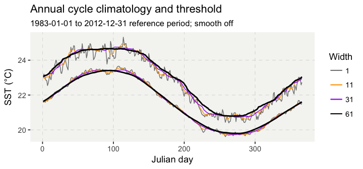
Figure 2. Daily climatologies of the mean (lower lines) and 90th percentile (top lines) produced by the detect() function, with various windowHalfWidth values and with smoothPercentile switched off.
To produce smoother climatologies, we can additionally enable a moving average smoother. The result is shown in Figure 3.
#smoothPercentile = TRUE
res.11.T <- ts2clm(sst_WA, climatologyPeriod = c("1983-01-01", "2012-12-31"), clmOnly = TRUE)
res.31.T <- ts2clm(sst_WA, climatologyPeriod = c("1983-01-01", "2012-12-31"), clmOnly = TRUE, windowHalfWidth = 15)
res.61.T <- ts2clm(sst_WA, climatologyPeriod = c("1983-01-01", "2012-12-31"), clmOnly = TRUE, windowHalfWidth = 30)res.11.T <- res.11.T %>%
mutate(width = "11")
res.31.T <- res.31.T %>%
mutate(width = "31")
res.61.T <- res.61.T %>%
mutate(width = "61")
smooth <- rbind(res.11.T, res.31.T, res.61.T)
plt2 <- ggplot(data = smooth,
aes(x = doy, y = seas)) +
geom_line(aes(colour = width, size = width)) +
geom_line(aes(y = thresh, colour = width, size = width)) +
scale_colour_manual(name = "Width",
values = c("orange", "purple", "black")) +
scale_size_manual(values = c(0.4, 0.4, 0.8), guide = FALSE) +
labs(x = "Julian day", y = "SST (°C)", title = "Annual cycle climatology and threshold",
subtitle = "1983-01-01 to 2012-12-31 reference period; smooth on") +
theme_publ()
ggsave(plt2, file = "climat_2.png", width = 6, height = 2.8, dpi = 120)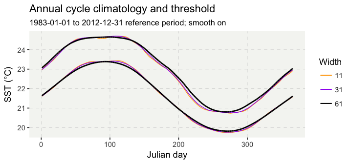
Figure 3. Daily climatologies of the mean (lower lines) and 90th percentile (upper lines) produced by the detect() function, with various windowHalfWidth values and with smoothPercentile at the default value of 31 days.
Fourier analysis of time series to construct a smooth climatology
library(fda)
clm <- res.1.F %>%
  as_tibble

b7 <- create.fourier.basis(rangeval = range(clm$doy), nbasis = 7)
# plot(b7)

# b7.val <- as_tibble(eval.basis(clm$doy, basisobj = b7))
# b7.val <- cbind(doy = clm$doy, b7.val) %>%
#   gather(key = "basis", value = "value", -doy) %>%
#   as_tibble()

# create smooth seasonal climatology
b7.seas.smth <- smooth.basis(argvals = clm$doy, y = clm$seas, fdParobj = b7)$fd
clm.seas.smth <- eval.fd(clm$doy, b7.seas.smth)

# create  smooth threshold
b7.thresh.smth <- smooth.basis(argvals = clm$doy, y = clm$thresh, fdParobj = b7)$fd
clm.thresh.smth <- eval.fd(clm$doy, b7.thresh.smth)

temps <- as_tibble(data.frame(doy = clm$doy,
                              seas.unsmth_1 = clm$seas,
                              seas.smth_11 = res.11.T$seas,
                              clim.fourier_7 = clm.seas.smth,
                              thresh.unsmth_1 = clm$thresh,
                              thresh.smth_11 = res.11.T$thresh,
thresh.fourier_7 = clm.thresh.smth))library(forcats)
plt3 <- temps %>%
gather(key = "type", value = "temperature", -doy) %>%
ggplot(aes(x = doy, y = temperature)) +
geom_line(aes(colour = fct_inorder(type), size = fct_inorder(type))) +
scale_colour_manual(name = "Smooth",
values = c("grey50", "purple", "black", "grey50", "purple", "black"),
labels = c("1, unsmooth", "11, smooth", "Fourier"),
breaks = c("seas.unsmth_1", "seas.smth_11", "clim.fourier_7")) +
scale_size_manual(values = c(0.4, 0.4, 0.8, 0.4, 0.4, 0.8), guide = FALSE) +
labs(x = "Julian day", y = "SST (°C)", title = "Annual cycle climatology and threshold",
subtitle = "1983-01-01 to 2012-12-31 reference period") +
theme_publ()
ggsave(plt3, file = "climat_3.png", width = 6, height = 2.8, dpi = 120)
# plot(b7.seas.smth[1:7])
# b7.PCA = pca.fd(b7.seas.smth, nharm=6)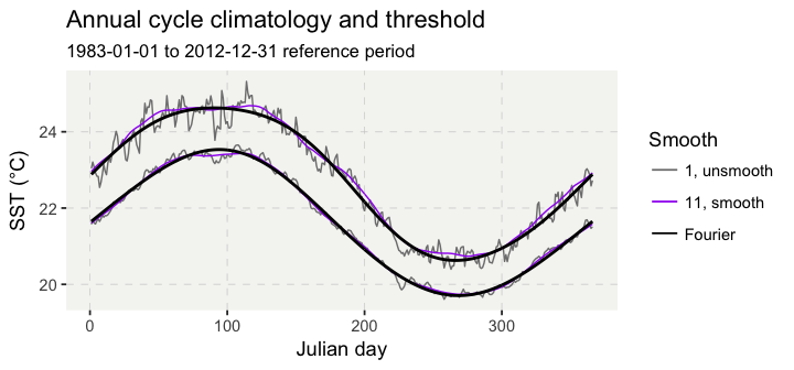
Figure 4. Daily climatologies of the mean (lower lines) and 90th percentile (upper lines) produced by the detect() function; “1, unsmooth” indicates that a windowHalfWidth of 0 days had been set, and that the data had not been subjected to smoothPercentile; “11, smooth” is the default settings of the detect() function; and “Fourier” indicates that an alternative climatology had been produced through the application of a Fourier analysis with 7 basis points.
# library(TSA)
# # compute the Fourier Transform
# p <- periodogram(y)
# dd <- data.frame(freq = p$freq, spec = p$spec)
# order <- dd[order(-dd$spec), ]
# top6 <- head(order, 6)
# # display the 6 highest "power" frequencies
# top6
# # convert frequency to time periods
# time <- 1/top6$f
# time
# fft(y)
# spectrum(y)# require(graphics)
# spec.y <- spec.pgram(y)
# plot(spec.y, plot.type = "coherency")
# plot(spec.y, plot.type = "phase")
# library(GeneCycle)
# GeneCycle::periodogram(y)Using a custom baseline
Should one want to use a different baseline to calculate the climatology against which the events should be detected, this is now possible.
# Again, using the built-in time series
# The Hobday et al. (2016) default definition applied above is available in
# `res.11.T`; we repeat it her and return the original time series with the
# climatology so as to have data in the specified format as required by the
# detect function, `detect_event()`:

res.11.T.full <- ts2clm(sst_WA, climatologyPeriod = c("1983-01-01", "2012-12-31"), clmOnly = FALSE)

# Calculate an anomaly:
daily.dat <- res.11.T.full %>%
  mutate(anom = temp - mean(temp, na.rm = TRUE),
         num = seq(1:length(temp)))

# Let us remove the long-term non-linear trend from the WA anomaly data using a
# generalised additive model; first, define the GAM:
library(mgcv)
library(broom)
mod.gam <- gam(temp ~ s(num, k = 20), data = daily.dat)
daily.dat2 <- augment(mod.gam)
daily.dat2 <- cbind(daily.dat2, daily.dat[, c("doy", "t", "anom")])

raw.clim <- ts2clm(daily.dat2, x = t, y = anom,
                   climatologyPeriod = c("1983-01-01", "2012-12-31"), clmOnly = FALSE)

detrended.clim <- ts2clm(daily.dat2, x = t, y = .resid,
                   climatologyPeriod = c("1983-01-01", "2012-12-31"), clmOnly = FALSE)

# Plot the two climatologies (raw vs. detrended):
plt4 <- ggplot(data = filter(raw.clim, t < "1983-01-01"), aes(x = doy, y = seas)) +
  geom_line(colour = "black") +
  geom_line(data = filter(detrended.clim, t < "1983-01-01"),
            colour = "red", alpha = 0.6) +
  theme_publ()
ggsave(plt4, file = "climat_4.png", width = 12, height = 6, dpi = 120)
# ... there is a tiny, almost imperceptable difference between the two...

# Calculate events in the original WA SST (anomaly) relative to a climatology
# created from the detrended WA SST data:
raw.res <- detect_event(raw.clim, x = t, y = anom,
                              seasClim = seas,
                              threshClim = thresh)

detrended.res <- detect_event(raw.clim, x = t, y = anom,
                              seasClim = detrended.clim$seas,
                              threshClim = detrended.clim$thresh)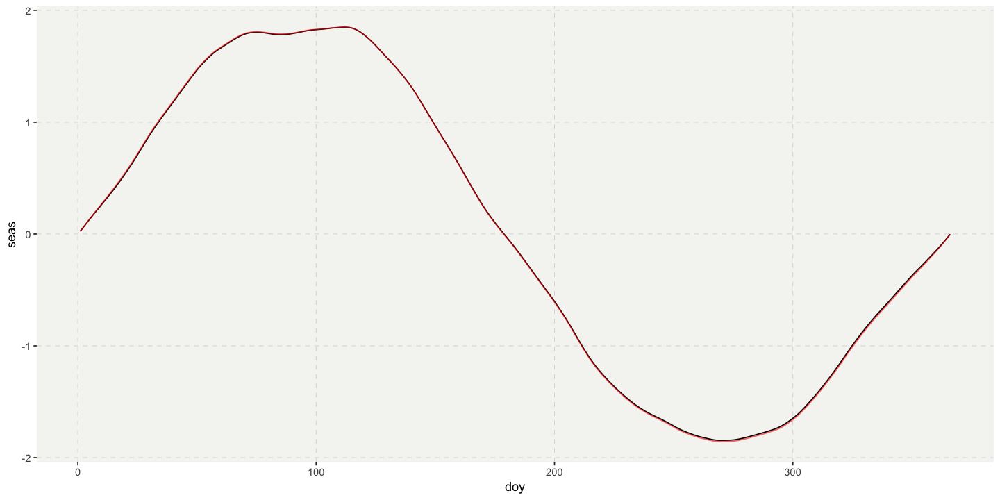
Figure 5. Daily climatologies of the WA SST (anomalies). The black line is the climatology prepared from the raw data, and the red line represents the daily SST anomalies that had been detrended using a generalised additive model. The lines plot practically on top of each other, so differences are barely perceptable; yet, despite these apparently small differences, there are large consequences for the events that are detected, as can be seen in the printout of the top 10 events, as seen below.
raw.resdetrended.resThe events that get detected are somewhat different now. Notice that in detrended.clim, seas and thresh are unfortunately the ones that were calculated together with raw (anomaly) time series, not the seas and thresh that were actually used and included against climSeas and climThresh. We will fix that.
Using a custom climatology
If one would rather supply a pre-calculated climatology, and not calculate one from a baseline, this is also now possible.
# Pull out the climatologies from the built in time series
# ts1_clim <- detect_evets2clm(sst_WA, climatologyPeriod = c("1983-01-01", "2012-12-31"))$clim %>%
#   dplyr::select(doy, seas, thresh, var_clim_year) %>%
#   base::unique() %>%
#   dplyr::arrange(doy)
# ts2_clim <- detect_evets2clm(sst_WA, climatologyPeriod = c("1983-01-01", "2012-12-31"))$clim %>%
#   dplyr::select(doy, seas, thresh, var_clim_year) %>%
#   base::unique() %>%
#   dplyr::arrange(doy)
# ts3_clim <- detect_evets2clm(sst_WA, climatologyPeriod = c("1983-01-01", "2012-12-31"))$clim %>%
#   dplyr::select(doy, seas, thresh, var_clim_year) %>%
#   base::unique() %>%
#   dplyr::arrange(doy)
#
# # Calculate events in one time series with a climatology from another
# res_clim_diff <- detect_event(ts1, alt_clim = TRUE, alt_clim_data = ts2_clim)
Note how the climatologies are the same below:
# head(ts2_clim)
# head(res_clim_diff$clim)
Should the provided climatology be to low, the function will return a warning letting the user know this.
# # Calculate events in one time series with a climatology from another
# res_clim_diff <- detect_event(ts1, alt_clim = TRUE, alt_clim_data = ts3_clim)