How to create climatologies from short time series
AJ Smit
2018-09-05
Short_climatologies.RmdHow does one create the best climatology? What if the time series is shorter than the recommended 30 years?
Lets look at all the SACTN data that’s longer than 30 years first. Can each site’s annual signal be represented by a sine/cosine curve derived from a Fourier analysis? First I find all the sites within the South African Coastal Temperature Network that are approximately 30 years or more in duration.
# load("~/SACTNraw/data/4_products/SACTN_daily_v4.2.RData")
load("/Volumes/GoogleDrive/My Drive/SACTN/SACTNraw/data/4_products/SACTN_daily_v4.2.RData")
daily.in <- SACTN_daily_v4.2
rm(SACTN_daily_v4.2)
long_sites <- daily.in %>%
  group_by(index) %>%
  summarise(n = n()) %>%
  filter(n >= 365 * 30) %>%
  ungroup()
Now, for each site that has ≥30 years of data, I create a daily climatology by taking the mean for each Julian day, using all data across the full duration of each time series.
daily <- daily.in %>%
  filter(index %in% long_sites$index) %>%
  mutate(index = as.character(index)) %>%
  # droplevels() %>%
  group_by(index) %>%
  mutate(doy = yday(date)) %>%
  group_by(index, doy) %>%
  summarise(temp = mean(temp, na.rm = TRUE)) %>%
  ungroup()
I make a function that will fit a Fourier series with seven basis functions (3 sine, 3 cosine and the constant) to the data. This is the same approach I used to create the smooth climatology in “Climatologies and baseline” elsewhere on this site, and it is also the one favoured in the creation of the daily Optimally Interpolated Sea Surface Temperature climatology (Banzon et al. 2014). Here it is wrapped in a function so I can easily apply it to each time series.
fFun <- function(data) {
  require(fda)
  b7 <- create.fourier.basis(rangeval = range(data$doy), nbasis = 7)

  # create smooth seasonal climatology
  b7.smth <- smooth.basis(argvals = data$doy, y = data$temp, fdParobj = b7)$fd
  data.smth <- eval.fd(data$doy, b7.smth)
  return(data.smth)
}
# currently this function fails when the 1st of January is an NA
# which sites have NAs?
excl.sites <- c(daily[is.na(daily$temp), 1])$index
daily.nest <- daily %>%
filter(!index %in% excl.sites) %>%
nest(-index)
daily.smth <- daily.nest %>%
mutate(smoothed = map(data, fFun)) %>%
unnest(data, smoothed)plt1 <- daily.smth %>%
ggplot(aes(x = doy, y = temp)) +
geom_point(shape = "+", colour = "red", alpha = 0.6, size = 1) +
geom_line(aes(y = smoothed, group = index), size = 0.6, colour = "black") +
facet_wrap(~index) +
labs(x = "Julian day", y = "Temperature (°C)", title = "SACTN: daily climatology",
subtitle = "Fourier series: 7 basis functions")
ggsave(plt1, file = "fig/SACTN_Fourier7.png", width = 12, height = 9, dpi = 120)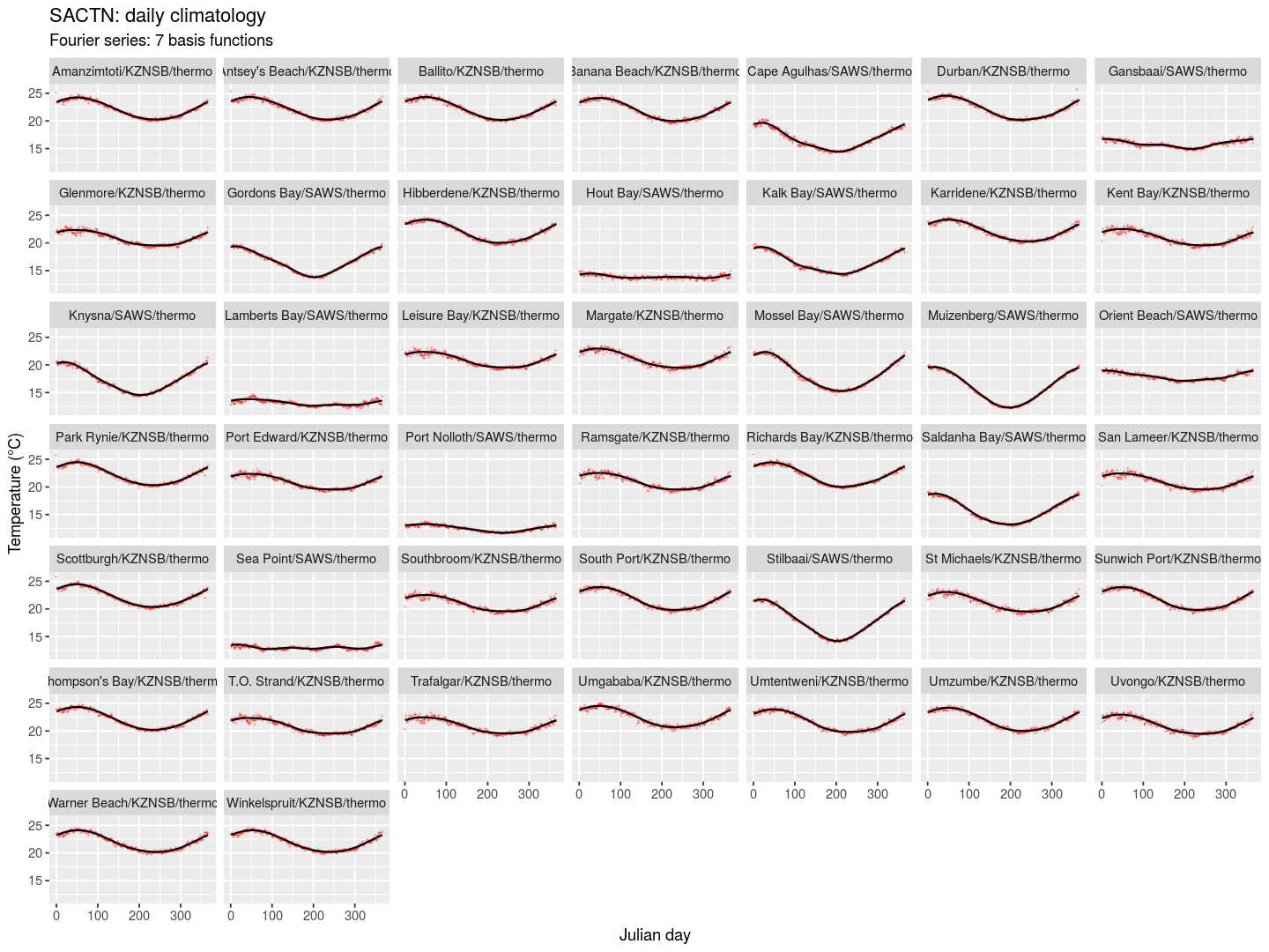
Figure 1. Smooth climatologies derived from a Fourier analysis fitted to coastal seawater time series along the South African coast. Climatologies were produced only for sites with at least 30 year long time series.
Time series length
Fourier series
There are instances when we might need to create climatologies when we don’t have access to time series of 30 years or longer. To look at this problem, I created a quick resampling analysis to see what the effect of time series length is on the resultant climatology. In this instance I used a Fourier analysis (see Banzon et al., 2014) to calculate six modes within an annual cycle, and used these to reconstruct a smooth climatology. This technique is quite forgiving of SST seasonalities that depart from typical sinusoidal profiles, such as which we find along upwelling areas (I have tested this on our coastal seawater temperatures).
I used the Western Australian data that’s packaged with the python and R marine heat wave scripts. Later I’ll test this more widely on other time series. The WA time series is 32 years long. I treat all temperatures over the duration of the time series as a pool of data, separately for each day-of-year (doy); i.e. doy 1 has 32 temperatures, doy 2 also has 32 temperatures, etc. I assume that the temperature on doy 1 of 1982 is independent of that on doy 1 in every other year (etc.), so the sample of doy 1 temperatures is therefore independent and identically distributed (i.i.d.). I further assume that there’s no autocorrelation from day-to-day (definitely erroneous, but I don’t think it matters here).
For each day’s pool of samples I then randomly take 10 samples and find the mean of that. This is the same as averaging over 10 years to obtain the mean for each of the 365 days (one year). Note that I did not apply the 11 day sliding window as per the heat wave function (windowHalfWidth), and rather opted to treat each doy independently as per Banzon et al. (2014). I repeat this 100 times, and so I effectively have estimates of a 100 annual cycles. I then do the same with 20 samples and 30 samples taken from the pool of available samples for each doy.
In total I now have 300 annual cycles: 100 of them representing a 10-year long times series, 100 representing a 20-year long time series, and 100 for a 30 year time series. To each of them, separately, I then fit the smooth climatology assembled from their Fourier components.
The attached plots show the outcome. The three panels represent 10, 20 and 30 year long time series. In Figure 2, each of the 100 daily time series is plotted as a line graph. In Figure 3, the red crosses show, for each doy, each of the 100 mean temperatures that I obtained. The black lines are of course the smooth climatologies–there is also 100 of these lines on each of the three panels.
So, using resampling and a Fourier analysis we can get away with using shorter time series. I can see later what happens if I shrink even further the time series down to only five years long. I will also test how well the python and R heatwave scripts’ internal climatology functions (windowHalfWidth and smoothPercentile) are able to produce reliable climatologies from short time series.
library(heatwaveR)
sst.in <- as_tibble(heatwaveR::sst_WA)
sst <- sst.in %>%
  mutate(doy = yday(as.Date(t))) %>%
  nest(-doy)

meanFun <- function(data) {
  m <- mean(data$temp, na.rm = TRUE)
  return(m)
}

sstRepl <- function(sst) {
  sst.sampled <- sst %>%
    mutate(sample_10 = map(data, sample_n, 10, replace = TRUE),
           sample_20 = map(data, sample_n, 20, replace = TRUE),
           sample_30 = map(data, sample_n, 30, replace = TRUE)) %>%
    mutate(sample_10_m = map(sample_10, meanFun),
           sample_20_m = map(sample_20, meanFun),
           sample_30_m = map(sample_30, meanFun)) %>%
    select(-data, -sample_10, -sample_20, -sample_30) %>%
    unnest(sample_10_m, sample_20_m, sample_30_m)
  return(sst.sampled)
}

library(purrr)
sst.repl <- purrr::rerun(100, sstRepl(sst)) %>%
  map_df(as.data.frame, .id = "rep") %>%
  gather(key = "ts.len", value = "temp", -rep, -doy)
plt2 <- ggplot(data = sst.repl, aes(x = doy, y = temp)) +
geom_line(aes(group = rep), alpha = 0.3, size = 0.1) +
facet_wrap(~ts.len, nrow = 3) +
labs(x = "Julian day", y = "SST (°C)", title = "Raw daily climatology",
subtitle = "100 daily climatological means")
ggsave(plt2, file = "fig/WA_100_simul.png", width = 12, height = 6, dpi = 120)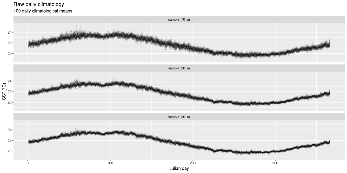
Figure 2. Resampled reconstructions of daily climatologies based on mean SSTs derived from time series fo 10, 20 and 30 years long. Each of 100 realisations are plotted as individual black traces on the three panels.
sst.repl.nest <- sst.repl %>%
  nest(-rep, -ts.len)

sst.repl.smth <- sst.repl.nest %>%
  mutate(smoothed = map(data, fFun)) %>%
  unnest(data, smoothed)
plt3 <- ggplot(data = sst.repl.smth, aes(x = doy, y = smoothed)) +
geom_point(aes(y = temp), shape = "+", colour = "red", alpha = 0.1, size = 1) +
geom_line(aes(group = rep), alpha = 0.3, size = 0.1) +
facet_wrap(~ts.len, nrow = 3) +
labs(x = "Julian day", y = "SST (°C)", title = "WA SST: daily climatology",
subtitle = "Fourier series: 7 basis functions")
ggsave(plt3, file = "fig/WA_Fourier7.png", width = 12, height = 6, dpi = 120)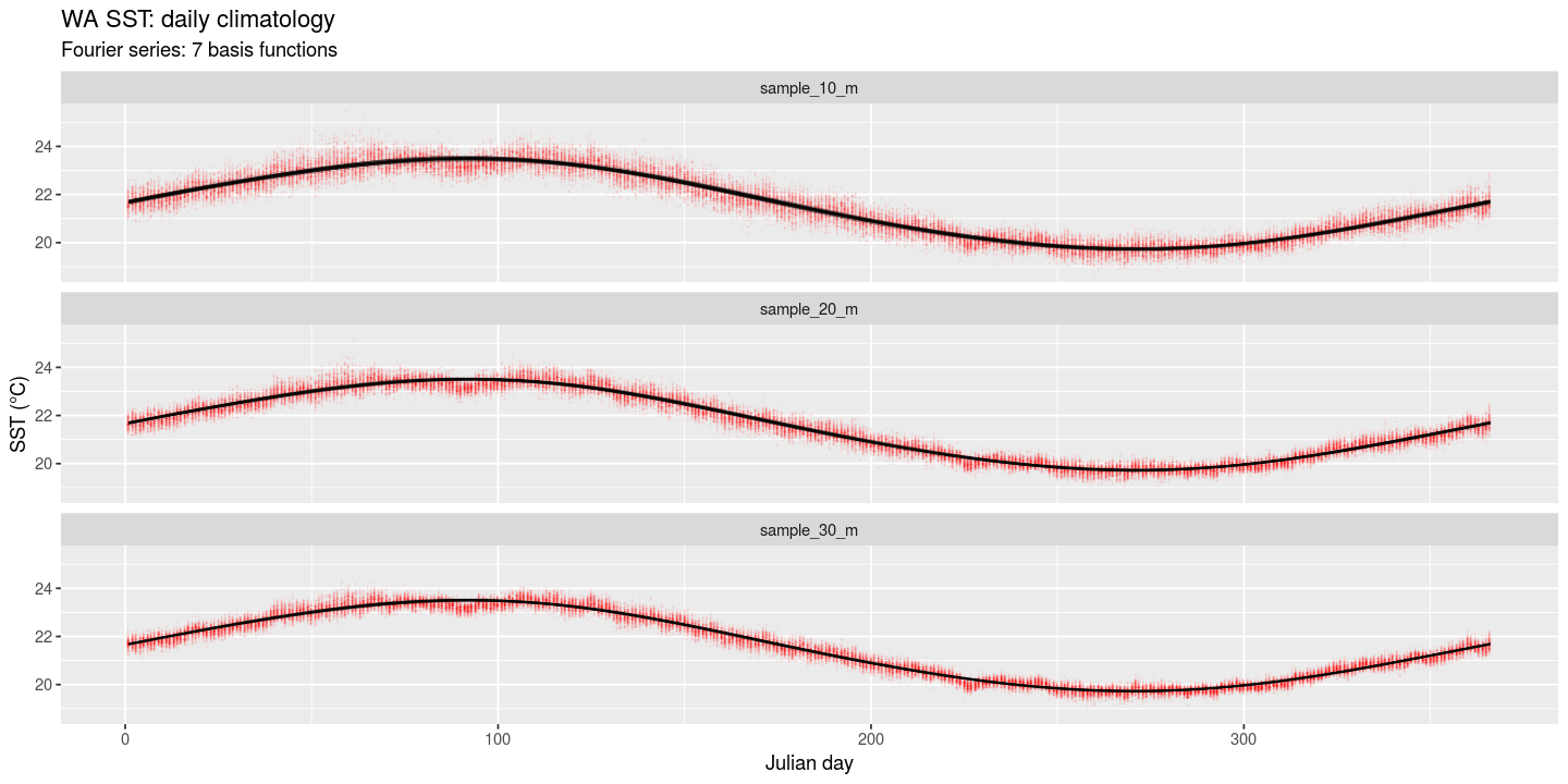
Figure 3. Resampled reconstructions of daily climatologies based on mean SSTs derived from time series of 10, 20 and 30 years long. Red lines are the smoothed climatologies obtained from a Fourier analysis.
heatwaveR’s climatology functions
The heatwaveR climatology tool creates the mean and 90th percentiles (threshold) for all the data within a sliding window with certain window width (by default 11 days centred on a day-of-year), and then this is followed by a running mean smoother for both the mean and the threshold. Using the approach I created for the Fourier series, lets do the same here.
sstRepl2 <- function(sst) {
  sst.sampled <- sst %>%
    mutate(sample_10 = map(data, sample_n, 10, replace = TRUE),
           sample_20 = map(data, sample_n, 20, replace = TRUE),
           sample_30 = map(data, sample_n, 30, replace = TRUE))
  return(sst.sampled)
}

sst.repl2 <- purrr::rerun(100, sstRepl2(sst)) %>%
  map_df(as.data.frame, .id = "rep")

parseDates <- function(data, rep_col, len) {
  parsed <- data %>%
    mutate(id = rep_col,
           y = year(t),
           m = month(t),
           d = day(t)) %>%
    group_by(rep, doy) %>%
    mutate(y = seq(1983, by = 1, len = len)) %>%
    mutate(t = ymd(paste(y, m, d, sep = "-"))) %>%
    select(-y, -m, -d) %>%
    na.omit() # because of complications due to leap years
  return(parsed)
}sample_10 <- sst.repl2 %>%
unnest(sample_10) %>%
parseDates("sample_10", len = 10) %>%
group_by(id, rep) %>%
nest() %>%
mutate(smoothed = map(data, function(x) ts2clm(x, climatologyPeriod = c("1983-01-01", "1992-12-31")))) %>%
unnest(smoothed)
sample_20 <- sst.repl2 %>%
unnest(sample_20) %>%
parseDates("sample_20", len = 20) %>%
group_by(id, rep) %>%
nest() %>%
mutate(smoothed = map(data, function(x) ts2clm(x, climatologyPeriod = c("1983-01-01", "2002-12-31")))) %>%
unnest(smoothed)
sample_30 <- sst.repl2 %>%
unnest(sample_30) %>%
parseDates("sample_30", len = 30) %>%
group_by(id, rep) %>%
nest() %>%
mutate(smoothed = map(data, function(x) ts2clm(x, climatologyPeriod = c("1983-01-01", "2012-12-31")))) %>%
unnest(smoothed)
sst.repl2.smth <- bind_rows(sample_10, sample_20, sample_30)plt4 <- sst.repl2.smth %>%
ggplot(aes(x = doy, y = temp)) +
# geom_point(shape = "+", colour = "red", alpha = 0.1, size = 1) +
geom_line(data = filter(sst.repl2.smth, t <= "1984-01-01"), aes(y = seas, group = rep), alpha = 0.3, size = 0.1) +
facet_wrap(~id, nrow = 3) +
labs(x = "Julian day", y = "SST (°C)", title = "WA SST: daily climatology",
subtitle = "MHW climatology, default settings")
ggsave(plt4, file = "fig/rand_mat_smoothed_2.png", width = 12, height = 6, dpi = 120)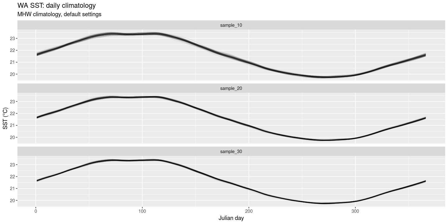
Figure 4. Resampled daily climatologies based on 10, 20 and 30 years long SST time series that were randomly assembled from the original 32-year long Western Australian SST data set included with the heatwaveR package. The lines are the smoothed climatologies obtained from applying the default heatwaveR climatology algorithm that includes a mean computed from all data withing a sliding 11-day wide window, centered on the doy, followed by a 31-day wide moving averages smoother.
Banzon, Viva F., Richard W. Reynolds, Diane Stokes, and Yan Xue. 2014. “A 1/4°-Spatial-resolution daily sea surface temperature climatology based on a blended satellite and in situ analysis.” Journal of Climate 27 (21): 8221–8. doi:10.1175/JCLI-D-14-00293.1.