<!DOCTYPE html>

<html xmlns="http://www.w3.org/1999/xhtml">

<head>

<meta charset="utf-8" />
<meta http-equiv="Content-Type" content="text/html; charset=utf-8" />
<meta name="generator" content="pandoc" />


<title>raster</title>

<script src="site_libs/jquery-1.11.3/jquery.min.js"></script>
<meta name="viewport" content="width=device-width, initial-scale=1" />
<link href="site_libs/bootstrap-3.3.5/css/cerulean.min.css" rel="stylesheet" />
<script src="site_libs/bootstrap-3.3.5/js/bootstrap.min.js"></script>
<script src="site_libs/bootstrap-3.3.5/shim/html5shiv.min.js"></script>
<script src="site_libs/bootstrap-3.3.5/shim/respond.min.js"></script>
<script src="site_libs/jqueryui-1.11.4/jquery-ui.min.js"></script>
<link href="site_libs/tocify-1.9.1/jquery.tocify.css" rel="stylesheet" />
<script src="site_libs/tocify-1.9.1/jquery.tocify.js"></script>
<script src="site_libs/navigation-1.1/tabsets.js"></script>
<link href="site_libs/font-awesome-5.0.13/css/fa-svg-with-js.css" rel="stylesheet" />
<script src="site_libs/font-awesome-5.0.13/js/fontawesome-all.min.js"></script>
<script src="site_libs/font-awesome-5.0.13/js/fa-v4-shims.min.js"></script>


<style type="text/css">code{white-space: pre;}</style>
<style type="text/css">
div.sourceCode { overflow-x: auto; }
table.sourceCode, tr.sourceCode, td.lineNumbers, td.sourceCode {
  margin: 0; padding: 0; vertical-align: baseline; border: none; }
table.sourceCode { width: 100%; line-height: 100%; background-color: #f8f8f8; }
td.lineNumbers { text-align: right; padding-right: 4px; padding-left: 4px; color: #aaaaaa; border-right: 1px solid #aaaaaa; }
td.sourceCode { padding-left: 5px; }
pre, code { background-color: #f8f8f8; }
code > span.kw { color: #204a87; font-weight: bold; } /* Keyword */
code > span.dt { color: #204a87; } /* DataType */
code > span.dv { color: #0000cf; } /* DecVal */
code > span.bn { color: #0000cf; } /* BaseN */
code > span.fl { color: #0000cf; } /* Float */
code > span.ch { color: #4e9a06; } /* Char */
code > span.st { color: #4e9a06; } /* String */
code > span.co { color: #8f5902; font-style: italic; } /* Comment */
code > span.ot { color: #8f5902; } /* Other */
code > span.al { color: #ef2929; } /* Alert */
code > span.fu { color: #000000; } /* Function */
code > span.er { color: #a40000; font-weight: bold; } /* Error */
code > span.wa { color: #8f5902; font-weight: bold; font-style: italic; } /* Warning */
code > span.cn { color: #000000; } /* Constant */
code > span.sc { color: #000000; } /* SpecialChar */
code > span.vs { color: #4e9a06; } /* VerbatimString */
code > span.ss { color: #4e9a06; } /* SpecialString */
code > span.im { } /* Import */
code > span.va { color: #000000; } /* Variable */
code > span.cf { color: #204a87; font-weight: bold; } /* ControlFlow */
code > span.op { color: #ce5c00; font-weight: bold; } /* Operator */
code > span.pp { color: #8f5902; font-style: italic; } /* Preprocessor */
code > span.ex { } /* Extension */
code > span.at { color: #c4a000; } /* Attribute */
code > span.do { color: #8f5902; font-weight: bold; font-style: italic; } /* Documentation */
code > span.an { color: #8f5902; font-weight: bold; font-style: italic; } /* Annotation */
code > span.cv { color: #8f5902; font-weight: bold; font-style: italic; } /* CommentVar */
code > span.in { color: #8f5902; font-weight: bold; font-style: italic; } /* Information */
</style>
<style type="text/css">
  pre:not([class]) {
    background-color: white;
  }
</style>


<style type="text/css">
h1 {
  font-size: 34px;
}
h1.title {
  font-size: 38px;
}
h2 {
  font-size: 30px;
}
h3 {
  font-size: 24px;
}
h4 {
  font-size: 18px;
}
h5 {
  font-size: 16px;
}
h6 {
  font-size: 12px;
}
.table th:not([align]) {
  text-align: left;
}
</style>


</head>

<body>

<style type = "text/css">
.main-container {
  max-width: 940px;
  margin-left: auto;
  margin-right: auto;
}
code {
  color: inherit;
  background-color: rgba(0, 0, 0, 0.04);
}
img {
  max-width:100%;
  height: auto;
}
.tabbed-pane {
  padding-top: 12px;
}
.html-widget {
  margin-bottom: 20px;
}
button.code-folding-btn:focus {
  outline: none;
}
</style>


<style type="text/css">
/* padding for bootstrap navbar */
body {
  padding-top: 51px;
  padding-bottom: 40px;
}
/* offset scroll position for anchor links (for fixed navbar)  */
.section h1 {
  padding-top: 56px;
  margin-top: -56px;
}

.section h2 {
  padding-top: 56px;
  margin-top: -56px;
}
.section h3 {
  padding-top: 56px;
  margin-top: -56px;
}
.section h4 {
  padding-top: 56px;
  margin-top: -56px;
}
.section h5 {
  padding-top: 56px;
  margin-top: -56px;
}
.section h6 {
  padding-top: 56px;
  margin-top: -56px;
}
</style>

<script>
// manage active state of menu based on current page
$(document).ready(function () {
  // active menu anchor
  href = window.location.pathname
  href = href.substr(href.lastIndexOf('/') + 1)
  if (href === "")
    href = "index.html";
  var menuAnchor = $('a[href="' + href + '"]');

  // mark it active
  menuAnchor.parent().addClass('active');

  // if it's got a parent navbar menu mark it active as well
  menuAnchor.closest('li.dropdown').addClass('active');
});
</script>


<div class="container-fluid main-container">

<!-- tabsets -->
<script>
$(document).ready(function () {
  window.buildTabsets("TOC");
});
</script>

<!-- code folding -->


<script>
$(document).ready(function ()  {

    // move toc-ignore selectors from section div to header
    $('div.section.toc-ignore')
        .removeClass('toc-ignore')
        .children('h1,h2,h3,h4,h5').addClass('toc-ignore');

    // establish options
    var options = {
      selectors: "h1,h2,h3",
      theme: "bootstrap3",
      context: '.toc-content',
      hashGenerator: function (text) {
        return text.replace(/[.\\/?&!#<>]/g, '').replace(/\s/g, '_').toLowerCase();
      },
      ignoreSelector: ".toc-ignore",
      scrollTo: 0
    };
    options.showAndHide = true;
    options.smoothScroll = true;

    // tocify
    var toc = $("#TOC").tocify(options).data("toc-tocify");
});
</script>

<style type="text/css">

#TOC {
  margin: 25px 0px 20px 0px;
}
@media (max-width: 768px) {
#TOC {
  position: relative;
  width: 100%;
}
}


.toc-content {
  padding-left: 30px;
  padding-right: 40px;
}

div.main-container {
  max-width: 1200px;
}

div.tocify {
  width: 20%;
  max-width: 260px;
  max-height: 85%;
}

@media (min-width: 768px) and (max-width: 991px) {
  div.tocify {
    width: 25%;
  }
}

@media (max-width: 767px) {
  div.tocify {
    width: 100%;
    max-width: none;
  }
}

.tocify ul, .tocify li {
  line-height: 20px;
}

.tocify-subheader .tocify-item {
  font-size: 0.90em;
  padding-left: 25px;
  text-indent: 0;
}

.tocify .list-group-item {
  border-radius: 0px;
}


</style>

<!-- setup 3col/9col grid for toc_float and main content  -->
<div class="row-fluid">
<div class="col-xs-12 col-sm-4 col-md-3">
<div id="TOC" class="tocify">
</div>
</div>

<div class="toc-content col-xs-12 col-sm-8 col-md-9">


<div class="navbar navbar-default  navbar-fixed-top" role="navigation">
  <div class="container">
    <div class="navbar-header">
      <button type="button" class="navbar-toggle collapsed" data-toggle="collapse" data-target="#navbar">
        <span class="icon-bar"></span>
        <span class="icon-bar"></span>
        <span class="icon-bar"></span>
      </button>
      <a class="navbar-brand" href="index.html">intro-r-gis</a>
    </div>
    <div id="navbar" class="navbar-collapse collapse">
      <ul class="nav navbar-nav">
        <li>
  <a href="index.html">Home</a>
</li>
<li>
  <a href="setup.html">Setup</a>
</li>
<li class="dropdown">
  <a href="#" class="dropdown-toggle" data-toggle="dropdown" role="button" aria-expanded="false">
    <span class="fa fa-gear"></span>
     
    Handouts
     
    <span class="caret"></span>
  </a>
  <ul class="dropdown-menu" role="menu">
    <li class="dropdown-header">Workshop Sections</li>
    <li>
      <a href="intro.html">Welcome</a>
    </li>
    <li>
      <a href="gis.html">Introduction to GIS</a>
    </li>
    <li>
      <a href="vector.html">Working with Vector Data</a>
    </li>
    <li>
      <a href="raster.html">Working with Raster Data</a>
    </li>
    <li class="divider"></li>
    <li>
      <a href="exercise_solutions.html">Exrecise solutions</a>
    </li>
  </ul>
</li>
      </ul>
      <ul class="nav navbar-nav navbar-right">
        <li>
  <a href="further_resources.html">Further Resources</a>
</li>
<li>
  <a href="https://github.com/annakrystalli/gis-workshop/archive/master.zip">Get Workshop Data</a>
</li>
<li>
  <a href="https://github.com/annakrystalli/intro-r-gis">
    <span class="fa fa-github"></span>
     
  </a>
</li>
      </ul>
    </div><!--/.nav-collapse -->
  </div><!--/.container -->
</div><!--/.navbar -->

<!-- Add a small amount of space between sections. -->
<style type="text/css">
div.section {
  padding-top: 12px;
}
</style>

<div class="fluid-row" id="header">


<h1 class="title toc-ignore">raster</h1>

</div>


<p><strong>Last updated:</strong> 2018-09-05</p>
<strong>workflowr checks:</strong> <small>(Click a bullet for more information)</small>
<ul>
<li>
<p><details> <summary> <strong style="color:blue;">✔</strong> <strong>R Markdown file:</strong> up-to-date </summary></p>
<p>Great! Since the R Markdown file has been committed to the Git repository, you know the exact version of the code that produced these results.</p>
</details>
</li>
<li>
<p><details> <summary> <strong style="color:blue;">✔</strong> <strong>Environment:</strong> empty </summary></p>
<p>Great job! The global environment was empty. Objects defined in the global environment can affect the analysis in your R Markdown file in unknown ways. For reproduciblity it’s best to always run the code in an empty environment.</p>
</details>
</li>
<li>
<p><details> <summary> <strong style="color:blue;">✔</strong> <strong>Seed:</strong> <code>set.seed(20180820)</code> </summary></p>
<p>The command <code>set.seed(20180820)</code> was run prior to running the code in the R Markdown file. Setting a seed ensures that any results that rely on randomness, e.g. subsampling or permutations, are reproducible.</p>
</details>
</li>
<li>
<p><details> <summary> <strong style="color:blue;">✔</strong> <strong>Session information:</strong> recorded </summary></p>
<p>Great job! Recording the operating system, R version, and package versions is critical for reproducibility.</p>
</details>
</li>
<li>
<p><details> <summary> <strong style="color:blue;">✔</strong> <strong>Repository version:</strong> <a href="https://github.com/annakrystalli/intro-r-gis/tree/5b425e1702224fa07d5ef7ab090dbb5ff32f8e21" target="_blank">5b425e1</a> </summary></p>
Great! You are using Git for version control. Tracking code development and connecting the code version to the results is critical for reproducibility. The version displayed above was the version of the Git repository at the time these results were generated. <br><br> Note that you need to be careful to ensure that all relevant files for the analysis have been committed to Git prior to generating the results (you can use <code>wflow_publish</code> or <code>wflow_git_commit</code>). workflowr only checks the R Markdown file, but you know if there are other scripts or data files that it depends on. Below is the status of the Git repository when the results were generated:
<pre><code>
Ignored files:
    Ignored:    .DS_Store
    Ignored:    .Rhistory
    Ignored:    .Rproj.user/
    Ignored:    analysis/.DS_Store
    Ignored:    analysis/assets/
    Ignored:    data-raw/
    Ignored:    data/csv/
    Ignored:    data/raster/
    Ignored:    data/sf/
    Ignored:    docs/.DS_Store

Untracked files:
    Untracked:  .Rbuildignore
    Untracked:  analysis/mapping.Rmd

Unstaged changes:
    Modified:   .gitignore
    Modified:   analysis/_site.yml
    Modified:   analysis/vector.Rmd

</code></pre>
Note that any generated files, e.g. HTML, png, CSS, etc., are not included in this status report because it is ok for generated content to have uncommitted changes. </details>
</li>
</ul>
<details> <summary> <small><strong>Expand here to see past versions:</strong></small> </summary>
<ul>
<table style="border-collapse:separate; border-spacing:5px;">
<thead>
<tr>
<th style="text-align:left;">
File
</th>
<th style="text-align:left;">
Version
</th>
<th style="text-align:left;">
Author
</th>
<th style="text-align:left;">
Date
</th>
<th style="text-align:left;">
Message
</th>
</tr>
</thead>
<tbody>
<tr>
<td style="text-align:left;">
Rmd
</td>
<td style="text-align:left;">
<a href="https://github.com/annakrystalli/intro-r-gis/blob/5b425e1702224fa07d5ef7ab090dbb5ff32f8e21/analysis/raster.Rmd" target="_blank">5b425e1</a>
</td>
<td style="text-align:left;">
annakrystalli
</td>
<td style="text-align:left;">
2018-09-05
</td>
<td style="text-align:left;">
workflowr::wflow_publish(c(“analysis/raster.Rmd”))
</td>
</tr>
<tr>
<td style="text-align:left;">
html
</td>
<td style="text-align:left;">
<a href="https://cdn.rawgit.com/annakrystalli/intro-r-gis/c91966eb061c8c7b7d8dbec843e427d1d673013d/docs/raster.html" target="_blank">c91966e</a>
</td>
<td style="text-align:left;">
annakrystalli
</td>
<td style="text-align:left;">
2018-09-05
</td>
<td style="text-align:left;">
Build site.
</td>
</tr>
<tr>
<td style="text-align:left;">
Rmd
</td>
<td style="text-align:left;">
<a href="https://github.com/annakrystalli/intro-r-gis/blob/9dd6ff79fcb120ffb6a977a35d9422cf6e8f4c76/analysis/raster.Rmd" target="_blank">9dd6ff7</a>
</td>
<td style="text-align:left;">
annakrystalli
</td>
<td style="text-align:left;">
2018-09-05
</td>
<td style="text-align:left;">
workflowr::wflow_publish(c(“analysis/raster.Rmd”))
</td>
</tr>
<tr>
<td style="text-align:left;">
html
</td>
<td style="text-align:left;">
<a href="https://cdn.rawgit.com/annakrystalli/intro-r-gis/0eb5925518bbc0ffb44e39ceb769d8bf7605b994/docs/raster.html" target="_blank">0eb5925</a>
</td>
<td style="text-align:left;">
annakrystalli
</td>
<td style="text-align:left;">
2018-09-05
</td>
<td style="text-align:left;">
Build site.
</td>
</tr>
<tr>
<td style="text-align:left;">
Rmd
</td>
<td style="text-align:left;">
<a href="https://github.com/annakrystalli/intro-r-gis/blob/a7080b8b1e1a1a2cb8c769c6defc04dc534f560f/analysis/raster.Rmd" target="_blank">a7080b8</a>
</td>
<td style="text-align:left;">
annakrystalli
</td>
<td style="text-align:left;">
2018-09-05
</td>
<td style="text-align:left;">
workflowr::wflow_publish(c(“analysis/raster.Rmd”))
</td>
</tr>
<tr>
<td style="text-align:left;">
html
</td>
<td style="text-align:left;">
<a href="https://cdn.rawgit.com/annakrystalli/intro-r-gis/88e2cb7dd0fb36fbd9df1593a44bef22187c0794/docs/raster.html" target="_blank">88e2cb7</a>
</td>
<td style="text-align:left;">
annakrystalli
</td>
<td style="text-align:left;">
2018-09-05
</td>
<td style="text-align:left;">
Build site.
</td>
</tr>
<tr>
<td style="text-align:left;">
html
</td>
<td style="text-align:left;">
<a href="https://cdn.rawgit.com/annakrystalli/intro-r-gis/42bd442c8a66face3bd1cd70b42915f6cba40983/docs/raster.html" target="_blank">42bd442</a>
</td>
<td style="text-align:left;">
annakrystalli
</td>
<td style="text-align:left;">
2018-09-04
</td>
<td style="text-align:left;">
Build site.
</td>
</tr>
<tr>
<td style="text-align:left;">
Rmd
</td>
<td style="text-align:left;">
<a href="https://github.com/annakrystalli/intro-r-gis/blob/8f5c11c5f7dbbb8751e64903a53e815ba3dd7870/analysis/raster.Rmd" target="_blank">8f5c11c</a>
</td>
<td style="text-align:left;">
annakrystalli
</td>
<td style="text-align:left;">
2018-09-04
</td>
<td style="text-align:left;">
workflowr::wflow_publish(“analysis/raster.Rmd”)
</td>
</tr>
<tr>
<td style="text-align:left;">
html
</td>
<td style="text-align:left;">
<a href="https://cdn.rawgit.com/annakrystalli/intro-r-gis/f94df5ce59f87379087af9763c9e1b64f7e9c0f3/docs/raster.html" target="_blank">f94df5c</a>
</td>
<td style="text-align:left;">
annakrystalli
</td>
<td style="text-align:left;">
2018-09-04
</td>
<td style="text-align:left;">
Build site.
</td>
</tr>
<tr>
<td style="text-align:left;">
Rmd
</td>
<td style="text-align:left;">
<a href="https://github.com/annakrystalli/intro-r-gis/blob/ae1fd63ac1f3d8a9f4792305b81ddcd208c5b515/analysis/raster.Rmd" target="_blank">ae1fd63</a>
</td>
<td style="text-align:left;">
annakrystalli
</td>
<td style="text-align:left;">
2018-09-04
</td>
<td style="text-align:left;">
workflowr::wflow_publish(c(“analysis/raster.Rmd”))
</td>
</tr>
</tbody>
</table>
</ul>
<p></details></p>
<hr />
<div id="setup" class="section level2">
<h2>setup</h2>
<div id="open-notebook" class="section level3">
<h3>Open Notebook</h3>
<p>Open a new <strong>R Notebook</strong> to work in.</p>
<blockquote>
<p>File &gt; New File &gt; R Notebook</p>
</blockquote>
<p>Name (eg. <code>Rasters</code>) and save it</p>
</div>
<div id="load-libraries" class="section level3">
<h3>Load libraries</h3>
<p>Load the libraries we’ll be using for this section of the workshop</p>
<div class="sourceCode"><pre class="sourceCode r"><code class="sourceCode r"><span class="kw">library</span>(raster)  
<span class="kw">library</span>(rasterVis)
<span class="kw">library</span>(sf)
<span class="kw">library</span>(dplyr)
<span class="kw">library</span>(ggplot2)</code></pre></div>
</div>
</div>
<div id="elements-of-raster-data" class="section level1">
<h1>Elements of raster data</h1>
<p>Gridded data. Each grid cell represented by pixels in the raster. Pixels represent an area of space on the Earth’s surface</p>
<p>3 core metadata elements: - Coordinate Reference System (CRS) - extent - resolution</p>
<p>See <a href="https://www.neonscience.org/raster-res-extent-pixels-r">“Raster resolution and extent”</a></p>
<div id="resolution" class="section level2">
<h2>Resolution</h2>
<p>The spatial resolution of a raster refers the size of each cell in meters. This size in turn relates to the area on the ground that the pixel represents.</p>
<div class="figure">
<img src="https://www.neonscience.org/sites/default/files/images/hyperspectral/pixelDetail.png" />

</div>
<p>The higher the resolution for the same extent the crisper the image (and the larger the file size) <img src="https://www.neonscience.org/sites/default/files/images/spatialData/raster1.png" /></p>
</div>
<div id="extent" class="section level2">
<h2>extent</h2>
<p><span class="math inline">\(x_{min} + (resolution_{x} \times n_{pixels}_{x})\)</span></p>
<div class="figure">
<img src="https://www.neonscience.org/sites/default/files/images/hyperspectral/sat_image_corners.png" />

</div>
<p>Unlike vector data, the raster data model stores the coordinate of the grid cell only indirectly: There is a less clear distinction between attribute and spatial information in raster data. Say, we are in the 3rd row and the 4th column of a raster matrix. To derive the corresponding coordinate, we have to move from the origin three cells in x-direction and four cells in y-direction with the cell resolution defining the distance for each x- and y-step.</p>
</div>
</div>
<div id="working-with-rasters" class="section level1">
<h1>Working with rasters</h1>
<div id="create-rasters" class="section level2">
<h2>Create rasters</h2>
<p>Rasters can be thought of as matrices appended with additional environmental metadata.</p>
<div class="sourceCode"><pre class="sourceCode r"><code class="sourceCode r">myRaster1 &lt;-<span class="st"> </span><span class="kw">raster</span>(<span class="dt">nrow=</span><span class="dv">4</span>, <span class="dt">ncol=</span><span class="dv">4</span>)
myRaster1</code></pre></div>
<pre><code>class       : RasterLayer 
dimensions  : 4, 4, 16  (nrow, ncol, ncell)
resolution  : 90, 45  (x, y)
extent      : -180, 180, -90, 90  (xmin, xmax, ymin, ymax)
coord. ref. : +proj=longlat +datum=WGS84 +ellps=WGS84 +towgs84=0,0,0 </code></pre>
<p>Let’s have a look at it. Note that when creating a raster, if not specified the CRS falls back to the defaults of:</p>
<ul>
<li>CRS: <code>+proj=longlat +datum=WGS84 +ellps=WGS84 +towgs84=0,0,0</code></li>
<li>extent: <code>-180, 180, -90, 90  (xmin, xmax, ymin, ymax)</code></li>
<li>resolution: <code>90, 45  (x, y)</code></li>
</ul>
<p>Q: What’s been defined?</p>
<p>Let’s give it some values</p>
<div class="sourceCode"><pre class="sourceCode r"><code class="sourceCode r">myRaster1[] &lt;-<span class="dv">1</span><span class="op">:</span><span class="dv">16</span>
<span class="kw">plot</span>(myRaster1)</code></pre></div>
<p><img src="figure/raster.Rmd/unnamed-chunk-3-1.png" width="672" style="display: block; margin: auto;" /></p>
<details> <summary><em>
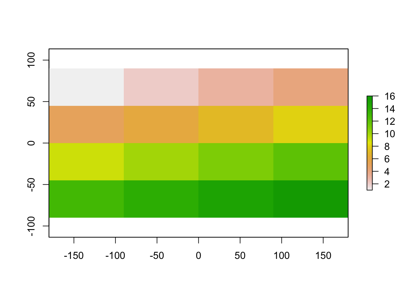
Expand here to see past versions of unnamed-chunk-3-1.png:</em></summary>
<table style="border-collapse:separate; border-spacing:5px;">
<thead>
<tr>
<th style="text-align:left;">
Version
</th>
<th style="text-align:left;">
Author
</th>
<th style="text-align:left;">
Date
</th>
</tr>
</thead>
<tbody>
<tr>
<td style="text-align:left;">
<a href="https://github.com/annakrystalli/intro-r-gis/blob/f94df5ce59f87379087af9763c9e1b64f7e9c0f3/docs/figure/raster.Rmd/unnamed-chunk-3-1.png" target="_blank">f94df5c</a>
</td>
<td style="text-align:left;">
annakrystalli
</td>
<td style="text-align:left;">
2018-09-04
</td>
</tr>
</tbody>
</table>
<p></details></p>
</div>
<div id="reading-raster-files" class="section level2">
<h2>Reading raster files</h2>
<div id="data" class="section level3">
<h3>Data</h3>
<div id="worldclim-data" class="section level4">
<h4><a href="http://www.worldclim.org/">WorldClim</a> data</h4>
<ul>
<li>A great resource of global environmental data in raster format.</li>
<li>Used extensively in species distribution modelling.</li>
<li>Version 2.0 available but not yet licensed under Creative Commons license (needed to redistribute this data for the workshop).</li>
<li>Was used in the Velo-Antón <em>et al</em> 2013 montane salamander paper!</li>
</ul>
</div>
<div id="bioclimatic-variables" class="section level4">
<h4><a href="http://www.worldclim.org/bioclim">Bioclimatic variables</a></h4>
<p>Bioclimatic variables are derived from the monthly temperature and rainfall values in order to generate more biologically meaningful variables. The bioclimatic variables represent annual trends, seasonality, and extreme or limiting environmental factors</p>
<ul>
<li>BIO1 = Annual Mean Temperature<br />
</li>
<li>BIO2 = Mean Diurnal Range (Mean of monthly (max temp - min temp))<br />
</li>
<li>BIO3 = Isothermality (BIO2/BIO7) (* 100)<br />
</li>
<li><strong>BIO4 = Temperature Seasonality (standard deviation *100)</strong><br />
</li>
<li><strong>BIO5 = Max Temperature of Warmest Month</strong><br />
</li>
<li><strong>BIO6 = Min Temperature of Coldest Month</strong><br />
</li>
<li>BIO7 = Temperature Annual Range (BIO5-BIO6)<br />
</li>
<li>BIO8 = Mean Temperature of Wettest Quarter<br />
</li>
<li>BIO9 = Mean Temperature of Driest Quarter<br />
</li>
<li>BIO10 = Mean Temperature of Warmest Quarter<br />
</li>
<li>BIO11 = Mean Temperature of Coldest Quarter<br />
</li>
<li>BIO12 = Annual Precipitation<br />
</li>
<li>BIO13 = Precipitation of Wettest Month<br />
</li>
<li>BIO14 = Precipitation of Driest Month<br />
</li>
<li><strong>BIO15 = Precipitation Seasonality (Coefficient of Variation)</strong><br />
</li>
<li>BIO16 = Precipitation of Wettest Quarter<br />
</li>
<li>BIO17 = Precipitation of Driest Quarter<br />
</li>
<li>BIO18 = Precipitation of Warmest Quarter<br />
</li>
<li>BIO19 = Precipitation of Coldest Quarter</li>
</ul>
<p>I’ve selected a few of the variables used in the original paper to fit a Species Distribution Model.</p>
<p>The data is in the <code>data/raster/mx-worldclim_30s</code> folder.</p>
<div class="sourceCode"><pre class="sourceCode r"><code class="sourceCode r">wc_files &lt;-<span class="st"> </span><span class="kw">list.files</span>(here<span class="op">::</span><span class="kw">here</span>(<span class="st">&quot;data&quot;</span>, <span class="st">&quot;raster&quot;</span>, <span class="st">&quot;mx-worldclim_30s&quot;</span>),
                       <span class="dt">full.names =</span> T)
wc_files</code></pre></div>
<pre><code>[1] &quot;/Users/Anna/Documents/workflows/workshops/intro-r-gis/data/raster/mx-worldclim_30s/mx-bio_15.tif&quot;
[2] &quot;/Users/Anna/Documents/workflows/workshops/intro-r-gis/data/raster/mx-worldclim_30s/mx-bio_4.tif&quot; 
[3] &quot;/Users/Anna/Documents/workflows/workshops/intro-r-gis/data/raster/mx-worldclim_30s/mx-bio_5.tif&quot; 
[4] &quot;/Users/Anna/Documents/workflows/workshops/intro-r-gis/data/raster/mx-worldclim_30s/mx-bio_6.tif&quot; </code></pre>
<p>These files are in <a href="https://en.wikipedia.org/wiki/GeoTIFF">GeoTIFF format</a>, a public domain metadata standard which allows georeferencing information to be embedded within a TIFF file.</p>
<p>Let’s start with a single raster file, <code>mx.bio_5.tif</code> which corresponds to <strong>bioclimatic variable 5: Max Temperature of Warmest Month</strong>.</p>
<div class="sourceCode"><pre class="sourceCode r"><code class="sourceCode r">bio5 &lt;-<span class="st"> </span><span class="kw">raster</span>(wc_files[<span class="dv">3</span>])
bio5</code></pre></div>
<pre><code>class       : RasterLayer 
dimensions  : 2181, 3638, 7934478  (nrow, ncol, ncell)
resolution  : 0.008333333, 0.008333333  (x, y)
extent      : -117.125, -86.80833, 14.54167, 32.71667  (xmin, xmax, ymin, ymax)
coord. ref. : +proj=longlat +datum=WGS84 +no_defs +ellps=WGS84 +towgs84=0,0,0 
data source : /Users/Anna/Documents/workflows/workshops/intro-r-gis/data/raster/mx-worldclim_30s/mx-bio_5.tif 
names       : mx.bio_5 
values      : 54, 427  (min, max)</code></pre>
<p>This creates a <code>RasterLayer</code> object.</p>
<p>By having a look at the summary of the raster file when we simply print the object, straight away it looks like something funny is going on. It’s showing a <strong>range of values between 54 and 427</strong>. Now, Mexico can get hot…but not that hot! By checking the <a href="http://www.worldclim.org/formats1">documentation</a> for the WorldClim data, we can see that the data is stored as <strong>degrees C x 10</strong>. This is for storage efficiency (files are much smaller if numbers can be stored as integers) but it means we need to transform the data back to degrees C.</p>
<p>Luckily we can easily manipulate rasters, just like any other matrix in R.</p>
<div class="sourceCode"><pre class="sourceCode r"><code class="sourceCode r">bio5 &lt;-<span class="st"> </span>bio5<span class="op">/</span><span class="dv">10</span>
bio5</code></pre></div>
<pre><code>class       : RasterLayer 
dimensions  : 2181, 3638, 7934478  (nrow, ncol, ncell)
resolution  : 0.008333333, 0.008333333  (x, y)
extent      : -117.125, -86.80833, 14.54167, 32.71667  (xmin, xmax, ymin, ymax)
coord. ref. : +proj=longlat +datum=WGS84 +no_defs +ellps=WGS84 +towgs84=0,0,0 
data source : in memory
names       : mx.bio_5 
values      : 5.4, 42.7  (min, max)</code></pre>
<p>That’s better!</p>
</div>
</div>
<div id="plotting-rasters" class="section level3">
<h3>Plotting rasters</h3>
<p>The <code>raster</code> pkg has native plotting functions which are again, ok for a quick check of the data.</p>
<div class="sourceCode"><pre class="sourceCode r"><code class="sourceCode r"><span class="kw">plot</span>(bio5)</code></pre></div>
<p><img src="figure/raster.Rmd/unnamed-chunk-7-1.png" width="672" style="display: block; margin: auto;" /></p>
<details> <summary><em>
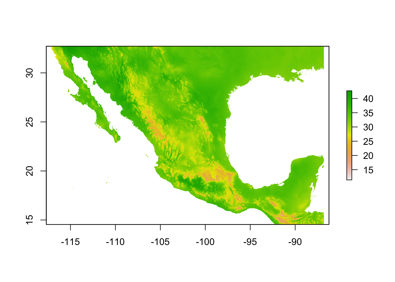
Expand here to see past versions of unnamed-chunk-7-1.png:</em></summary>
<table style="border-collapse:separate; border-spacing:5px;">
<thead>
<tr>
<th style="text-align:left;">
Version
</th>
<th style="text-align:left;">
Author
</th>
<th style="text-align:left;">
Date
</th>
</tr>
</thead>
<tbody>
<tr>
<td style="text-align:left;">
<a href="https://github.com/annakrystalli/intro-r-gis/blob/f94df5ce59f87379087af9763c9e1b64f7e9c0f3/docs/figure/raster.Rmd/unnamed-chunk-7-1.png" target="_blank">f94df5c</a>
</td>
<td style="text-align:left;">
annakrystalli
</td>
<td style="text-align:left;">
2018-09-04
</td>
</tr>
</tbody>
</table>
<p></details></p>
<p>Package <code>rasterVis</code> offers much nicer options for plotting raster data, including much better colour palletes which are pretty, better represent data, are easier to read by those with colorblindness, and print well in grey scale. by default.</p>
<div class="sourceCode"><pre class="sourceCode r"><code class="sourceCode r"><span class="kw">levelplot</span>(bio5)</code></pre></div>
<p><img src="figure/raster.Rmd/unnamed-chunk-8-1.png" width="672" style="display: block; margin: auto;" /></p>
<details> <summary><em>
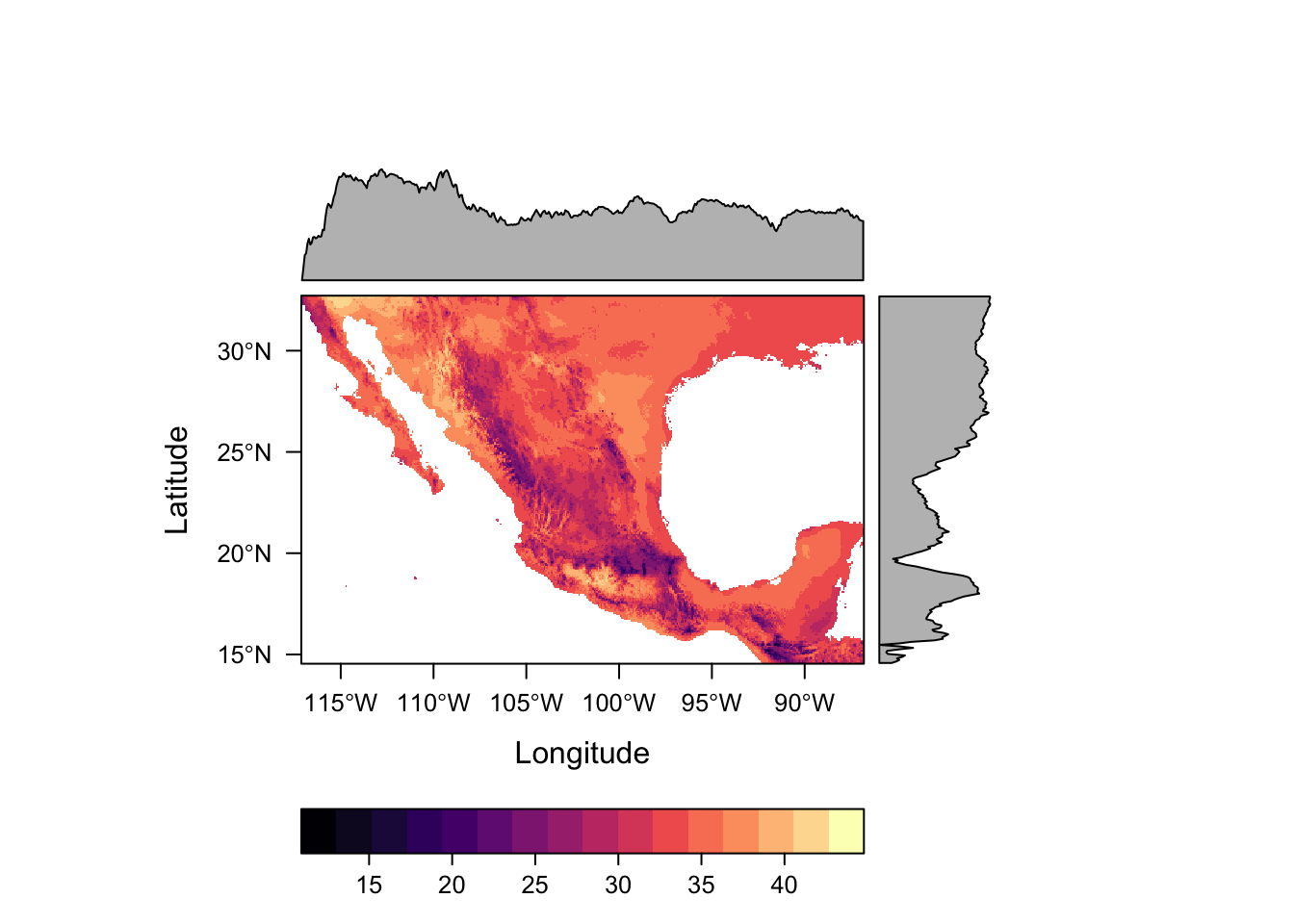
Expand here to see past versions of unnamed-chunk-8-1.png:</em></summary>
<table style="border-collapse:separate; border-spacing:5px;">
<thead>
<tr>
<th style="text-align:left;">
Version
</th>
<th style="text-align:left;">
Author
</th>
<th style="text-align:left;">
Date
</th>
</tr>
</thead>
<tbody>
<tr>
<td style="text-align:left;">
<a href="https://github.com/annakrystalli/intro-r-gis/blob/f94df5ce59f87379087af9763c9e1b64f7e9c0f3/docs/figure/raster.Rmd/unnamed-chunk-8-1.png" target="_blank">f94df5c</a>
</td>
<td style="text-align:left;">
annakrystalli
</td>
<td style="text-align:left;">
2018-09-04
</td>
</tr>
</tbody>
</table>
<p></details></p>
<p>For numeric data it plots the distribution of the data along each axis in the plot margins. We can suppress that default behaviour by using argument <code>margin=FALSE</code>.</p>
<div class="sourceCode"><pre class="sourceCode r"><code class="sourceCode r"><span class="kw">levelplot</span>(bio5, <span class="dt">margin=</span><span class="ot">FALSE</span>)</code></pre></div>
<p><img src="figure/raster.Rmd/unnamed-chunk-9-1.png" width="672" style="display: block; margin: auto;" /></p>
<details> <summary><em>
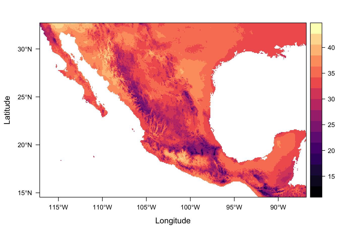
Expand here to see past versions of unnamed-chunk-9-1.png:</em></summary>
<table style="border-collapse:separate; border-spacing:5px;">
<thead>
<tr>
<th style="text-align:left;">
Version
</th>
<th style="text-align:left;">
Author
</th>
<th style="text-align:left;">
Date
</th>
</tr>
</thead>
<tbody>
<tr>
<td style="text-align:left;">
<a href="https://github.com/annakrystalli/intro-r-gis/blob/f94df5ce59f87379087af9763c9e1b64f7e9c0f3/docs/figure/raster.Rmd/unnamed-chunk-9-1.png" target="_blank">f94df5c</a>
</td>
<td style="text-align:left;">
annakrystalli
</td>
<td style="text-align:left;">
2018-09-04
</td>
</tr>
</tbody>
</table>
<p></details></p>
<p>Now this is great for individual layers, but if we have multiple layers to work with, it can be much more efficient to <strong>stack</strong> them into a <code>rasterStack</code>.</p>
</div>
<div id="raster-stacks" class="section level3">
<h3>Raster Stacks</h3>
<p>A <code>RasterStack</code> is a <strong>collection of RasterLayer objects with the same spatial extent and resolution</strong>. A RasterStack can be created from <code>RasterLayer</code> objects, or from raster files, or both.</p>
<p>We can read and stack raster files in one go using function <code>raster::stack</code>! And this is where the list of file names comes in handy.</p>
<div class="sourceCode"><pre class="sourceCode r"><code class="sourceCode r">st &lt;-<span class="st"> </span><span class="kw">stack</span>(wc_files) 

st</code></pre></div>
<pre><code>class       : RasterStack 
dimensions  : 2181, 3638, 7934478, 4  (nrow, ncol, ncell, nlayers)
resolution  : 0.008333333, 0.008333333  (x, y)
extent      : -117.125, -86.80833, 14.54167, 32.71667  (xmin, xmax, ymin, ymax)
coord. ref. : +proj=longlat +datum=WGS84 +no_defs +ellps=WGS84 +towgs84=0,0,0 
names       : mx.bio_15, mx.bio_4, mx.bio_5, mx.bio_6 
min values  :        10,      199,       54,      -85 
max values  :       140,     8136,      427,      218 </code></pre>
<p>We can still extract individual layers using function <code>raster::subset()</code>.</p>
<div class="sourceCode"><pre class="sourceCode r"><code class="sourceCode r"><span class="kw">subset</span>(st, <span class="st">&quot;mx.bio_5&quot;</span>)</code></pre></div>
<pre><code>class       : RasterLayer 
dimensions  : 2181, 3638, 7934478  (nrow, ncol, ncell)
resolution  : 0.008333333, 0.008333333  (x, y)
extent      : -117.125, -86.80833, 14.54167, 32.71667  (xmin, xmax, ymin, ymax)
coord. ref. : +proj=longlat +datum=WGS84 +no_defs +ellps=WGS84 +towgs84=0,0,0 
data source : /Users/Anna/Documents/workflows/workshops/intro-r-gis/data/raster/mx-worldclim_30s/mx-bio_5.tif 
names       : mx.bio_5 
values      : 54, 427  (min, max)</code></pre>
<p>Because a <code>rasterStack</code> is effectively a list, we can also subset it as we would any other list in R</p>
<div class="sourceCode"><pre class="sourceCode r"><code class="sourceCode r">st[[<span class="st">&quot;mx.bio_5&quot;</span>]]</code></pre></div>
<pre><code>class       : RasterLayer 
dimensions  : 2181, 3638, 7934478  (nrow, ncol, ncell)
resolution  : 0.008333333, 0.008333333  (x, y)
extent      : -117.125, -86.80833, 14.54167, 32.71667  (xmin, xmax, ymin, ymax)
coord. ref. : +proj=longlat +datum=WGS84 +no_defs +ellps=WGS84 +towgs84=0,0,0 
data source : /Users/Anna/Documents/workflows/workshops/intro-r-gis/data/raster/mx-worldclim_30s/mx-bio_5.tif 
names       : mx.bio_5 
values      : 54, 427  (min, max)</code></pre>
<div class="sourceCode"><pre class="sourceCode r"><code class="sourceCode r">st[[<span class="dv">3</span>]]</code></pre></div>
<pre><code>class       : RasterLayer 
dimensions  : 2181, 3638, 7934478  (nrow, ncol, ncell)
resolution  : 0.008333333, 0.008333333  (x, y)
extent      : -117.125, -86.80833, 14.54167, 32.71667  (xmin, xmax, ymin, ymax)
coord. ref. : +proj=longlat +datum=WGS84 +no_defs +ellps=WGS84 +towgs84=0,0,0 
data source : /Users/Anna/Documents/workflows/workshops/intro-r-gis/data/raster/mx-worldclim_30s/mx-bio_5.tif 
names       : mx.bio_5 
values      : 54, 427  (min, max)</code></pre>
<p>Note that we are back to having incorrect temperature values. We will deal with the layers that need correcting a bit later so just ignore that for now.</p>
<p>Both the native <code>plot</code> method and <code>rasterVis::levelplot</code> can handle <code>rasterStack</code>s</p>
<div class="sourceCode"><pre class="sourceCode r"><code class="sourceCode r"><span class="kw">plot</span>(st)</code></pre></div>
<p><img src="figure/raster.Rmd/unnamed-chunk-14-1.png" width="672" style="display: block; margin: auto;" /></p>
<details> <summary><em>
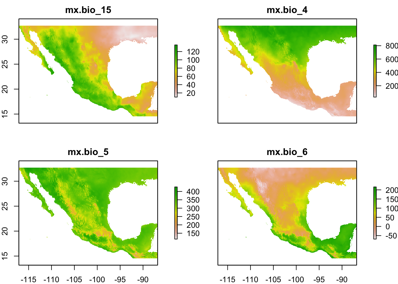
Expand here to see past versions of unnamed-chunk-14-1.png:</em></summary>
<table style="border-collapse:separate; border-spacing:5px;">
<thead>
<tr>
<th style="text-align:left;">
Version
</th>
<th style="text-align:left;">
Author
</th>
<th style="text-align:left;">
Date
</th>
</tr>
</thead>
<tbody>
<tr>
<td style="text-align:left;">
<a href="https://github.com/annakrystalli/intro-r-gis/blob/f94df5ce59f87379087af9763c9e1b64f7e9c0f3/docs/figure/raster.Rmd/unnamed-chunk-14-1.png" target="_blank">f94df5c</a>
</td>
<td style="text-align:left;">
annakrystalli
</td>
<td style="text-align:left;">
2018-09-04
</td>
</tr>
</tbody>
</table>
<p></details></p>
<div class="sourceCode"><pre class="sourceCode r"><code class="sourceCode r"><span class="kw">levelplot</span>(st)</code></pre></div>
<p><img src="figure/raster.Rmd/unnamed-chunk-15-1.png" width="672" style="display: block; margin: auto;" /></p>
<details> <summary><em>
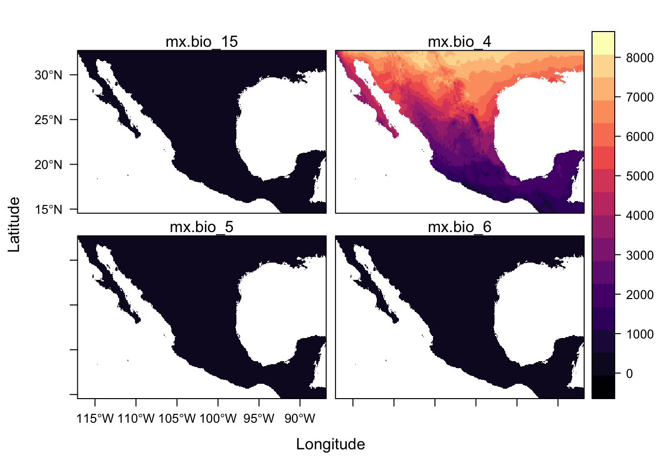
Expand here to see past versions of unnamed-chunk-15-1.png:</em></summary>
<table style="border-collapse:separate; border-spacing:5px;">
<thead>
<tr>
<th style="text-align:left;">
Version
</th>
<th style="text-align:left;">
Author
</th>
<th style="text-align:left;">
Date
</th>
</tr>
</thead>
<tbody>
<tr>
<td style="text-align:left;">
<a href="https://github.com/annakrystalli/intro-r-gis/blob/f94df5ce59f87379087af9763c9e1b64f7e9c0f3/docs/figure/raster.Rmd/unnamed-chunk-15-1.png" target="_blank">f94df5c</a>
</td>
<td style="text-align:left;">
annakrystalli
</td>
<td style="text-align:left;">
2018-09-04
</td>
</tr>
</tbody>
</table>
<p></details></p>
<p>For a quick scan of a <code>rasterStack</code>, <code>plot()</code> is more useful because <code>levelplot()</code> function plot all panels on the same scale but there are ways of plotting with separate scales which we will link to later.</p>
</div>
<div id="landcover-data" class="section level3">
<h3>Landcover data</h3>
<p>Land cover, original data resampled onto a 30 seconds grid sourced from <a href="http://www.diva-gis.org/gdata">DIVA GIS</a>. DIVA-GIS is a free computer program for mapping and geographic data analysis (a geographic information system (GIS) which also provide free global spatial data.</p>
<div class="sourceCode"><pre class="sourceCode r"><code class="sourceCode r">lc_files &lt;-<span class="st"> </span><span class="kw">list.files</span>(here<span class="op">::</span><span class="kw">here</span>(<span class="st">&quot;data&quot;</span>, <span class="st">&quot;raster&quot;</span>, <span class="st">&quot;MEX_msk_cov&quot;</span>),
                       <span class="dt">full.names =</span> T)</code></pre></div>
<div class="sourceCode"><pre class="sourceCode r"><code class="sourceCode r">lc &lt;-<span class="st"> </span><span class="kw">raster</span>(lc_files[<span class="dv">1</span>])
lc</code></pre></div>
<pre><code>class       : RasterLayer 
dimensions  : 2208, 3696, 8160768  (nrow, ncol, ncell)
resolution  : 0.008333333, 0.008333333  (x, y)
extent      : -117.4, -86.6, 14.4, 32.8  (xmin, xmax, ymin, ymax)
coord. ref. : +proj=longlat +ellps=WGS84 
data source : /Users/Anna/Documents/workflows/workshops/intro-r-gis/data/raster/MEX_msk_cov/MEX_msk_cov.grd 
names       : MEX_msk_cov 
values      : 1, 22  (min, max)</code></pre>
<p>Let’s plot this again to have a look at it.</p>
<div class="sourceCode"><pre class="sourceCode r"><code class="sourceCode r"><span class="kw">levelplot</span>(lc)</code></pre></div>
<p><img src="figure/raster.Rmd/unnamed-chunk-18-1.png" width="672" style="display: block; margin: auto;" /></p>
<details> <summary><em>
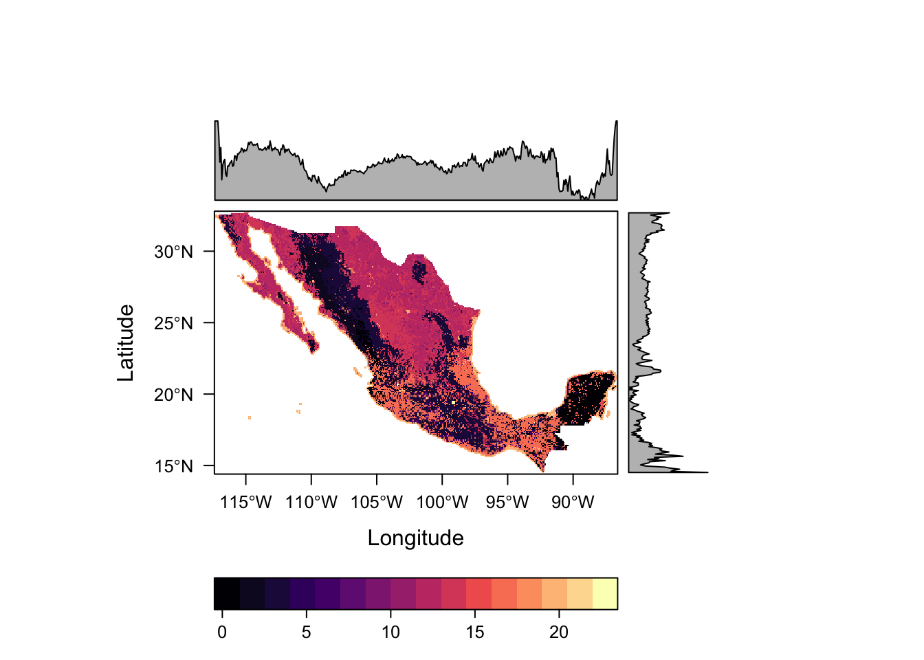
Expand here to see past versions of unnamed-chunk-18-1.png:</em></summary>
<table style="border-collapse:separate; border-spacing:5px;">
<thead>
<tr>
<th style="text-align:left;">
Version
</th>
<th style="text-align:left;">
Author
</th>
<th style="text-align:left;">
Date
</th>
</tr>
</thead>
<tbody>
<tr>
<td style="text-align:left;">
<a href="https://github.com/annakrystalli/intro-r-gis/blob/f94df5ce59f87379087af9763c9e1b64f7e9c0f3/docs/figure/raster.Rmd/unnamed-chunk-18-1.png" target="_blank">f94df5c</a>
</td>
<td style="text-align:left;">
annakrystalli
</td>
<td style="text-align:left;">
2018-09-04
</td>
</tr>
</tbody>
</table>
<p></details></p>
<p>This raster contains categorical data, so the scales used as well as the inclusion of distributions along the margins do not see appropriate. Such data can be better defined using the <code>rasteVis::ratify</code> function.</p>
<div class="sourceCode"><pre class="sourceCode r"><code class="sourceCode r">lc &lt;-<span class="st"> </span><span class="kw">ratify</span>(lc)
lc</code></pre></div>
<pre><code>class       : RasterLayer 
dimensions  : 2208, 3696, 8160768  (nrow, ncol, ncell)
resolution  : 0.008333333, 0.008333333  (x, y)
extent      : -117.4, -86.6, 14.4, 32.8  (xmin, xmax, ymin, ymax)
coord. ref. : +proj=longlat +ellps=WGS84 
data source : /Users/Anna/Documents/workflows/workshops/intro-r-gis/data/raster/MEX_msk_cov/MEX_msk_cov.grd 
names       : MEX_msk_cov 
values      : 1, 22  (min, max)
attributes  :
       ID
 from:  1
 to  : 22</code></pre>
<p>Now we see that rather than a <code>values: 1, 22  (min, max)</code> we have an <code>attributes:</code> field containing a table summarising the levels with <code>from:</code> for the first and <code>to:</code> for the last entry. The actual levels are stored in what is known as a <strong>“Raster Attribute Table” (RAT)</strong>. This can be accessed through the <code>levels()</code> function.</p>
<div class="sourceCode"><pre class="sourceCode r"><code class="sourceCode r"><span class="kw">levels</span>(lc)</code></pre></div>
<pre><code>[[1]]
   ID
1   1
2   2
3   4
4   6
5   9
6  11
7  12
8  13
9  14
10 15
11 16
12 20
13 22</code></pre>
<p>Let’s try and plot again.</p>
<div class="sourceCode"><pre class="sourceCode r"><code class="sourceCode r"><span class="kw">levelplot</span>(lc)</code></pre></div>
<pre><code>Error in `[.data.frame`(rat, , att): undefined columns selected</code></pre>
<p>This time, plotting fails. This is because there are no descriptions associated with the levels.</p>
<p>We can define this defined with more informative descriptions. As I forgot to save them as <code>.csv</code> as part of the workshop materials, here is a snippet of code that can be copied and pasted to create a data.frame of factor levels and their associated descriptions.</p>
<p>(or go to <a href="http://bit.ly/lc_levels" class="uri">http://bit.ly/lc_levels</a>, click on raw and copy the code snippet from there)</p>
<div class="sourceCode"><pre class="sourceCode r"><code class="sourceCode r">lc_levels &lt;-<span class="st"> </span><span class="kw">structure</span>(<span class="kw">list</span>(<span class="dt">level =</span> <span class="dv">1</span><span class="op">:</span><span class="dv">22</span>, <span class="dt">descr =</span> <span class="kw">c</span>(<span class="st">&quot;Tree Cover, broadleaved, evergreen&quot;</span>, 
<span class="st">&quot;Tree Cover, broadleaved, deciduous, closed&quot;</span>, <span class="st">&quot;Tree Cover, broadleaved, deciduous, open&quot;</span>, 
<span class="st">&quot;Tree Cover, needle-leaved, evergreen&quot;</span>, <span class="st">&quot;Tree Cover, needle-leaved, deciduous&quot;</span>, 
<span class="st">&quot;Tree Cover, mixed leaf type&quot;</span>, <span class="st">&quot;Tree Cover, regularly flooded, fresh  water&quot;</span>, 
<span class="st">&quot;Tree Cover, regularly flooded, saline water&quot;</span>, <span class="st">&quot;Mosaic: Tree cover / Other natural vegetation&quot;</span>, 
<span class="st">&quot;Tree Cover, burnt&quot;</span>, <span class="st">&quot;Shrub Cover, closed-open, evergreen&quot;</span>, <span class="st">&quot;Shrub Cover, closed-open, deciduous&quot;</span>, 
<span class="st">&quot;Herbaceous Cover, closed-open&quot;</span>, <span class="st">&quot;Sparse Herbaceous or sparse Shrub Cover&quot;</span>, 
<span class="st">&quot;Regularly flooded Shrub and/or Herbaceous Cover&quot;</span>, <span class="st">&quot;Cultivated and managed areas&quot;</span>, 
<span class="st">&quot;Mosaic: Cropland / Tree Cover / Other natural vegetation&quot;</span>, <span class="st">&quot;Mosaic: Cropland / Shrub or Grass Cover&quot;</span>, 
<span class="st">&quot;Bare Areas&quot;</span>, <span class="st">&quot;Water Bodies&quot;</span>, <span class="st">&quot;Snow and Ice&quot;</span>, <span class="st">&quot;Artificial surfaces and associated areas&quot;</span>
)), <span class="dt">class =</span> <span class="st">&quot;data.frame&quot;</span>, <span class="dt">.Names =</span> <span class="kw">c</span>(<span class="st">&quot;level&quot;</span>, <span class="st">&quot;descr&quot;</span>), <span class="dt">row.names =</span> <span class="kw">c</span>(<span class="ot">NA</span>, 
<span class="op">-</span>22L))</code></pre></div>
<div class="sourceCode"><pre class="sourceCode r"><code class="sourceCode r">rat &lt;-<span class="st"> </span><span class="kw">levels</span>(lc)[[<span class="dv">1</span>]]
rat &lt;-<span class="st"> </span>rat <span class="op">%&gt;%</span><span class="st"> </span><span class="kw">left_join</span>(lc_levels, <span class="dt">by =</span> <span class="kw">c</span>(<span class="st">&quot;ID&quot;</span> =<span class="st"> &quot;level&quot;</span>))
<span class="kw">levels</span>(lc) &lt;-<span class="st"> </span>rat</code></pre></div>
<p>Let’s have a look at our land cover raster</p>
<div class="sourceCode"><pre class="sourceCode r"><code class="sourceCode r">lc</code></pre></div>
<pre><code>class       : RasterLayer 
dimensions  : 2208, 3696, 8160768  (nrow, ncol, ncell)
resolution  : 0.008333333, 0.008333333  (x, y)
extent      : -117.4, -86.6, 14.4, 32.8  (xmin, xmax, ymin, ymax)
coord. ref. : +proj=longlat +ellps=WGS84 
data source : /Users/Anna/Documents/workflows/workshops/intro-r-gis/data/raster/MEX_msk_cov/MEX_msk_cov.grd 
names       : MEX_msk_cov 
values      : 1, 22  (min, max)
attributes  :
       ID                                    descr
 from:  1       Tree Cover, broadleaved, evergreen
 to  : 22 Artificial surfaces and associated areas</code></pre>
<p>Let’s plot again</p>
<div class="sourceCode"><pre class="sourceCode r"><code class="sourceCode r"><span class="kw">levelplot</span>(lc)</code></pre></div>
<p><img src="figure/raster.Rmd/unnamed-chunk-25-1.png" width="672" style="display: block; margin: auto;" /></p>
<details> <summary><em>
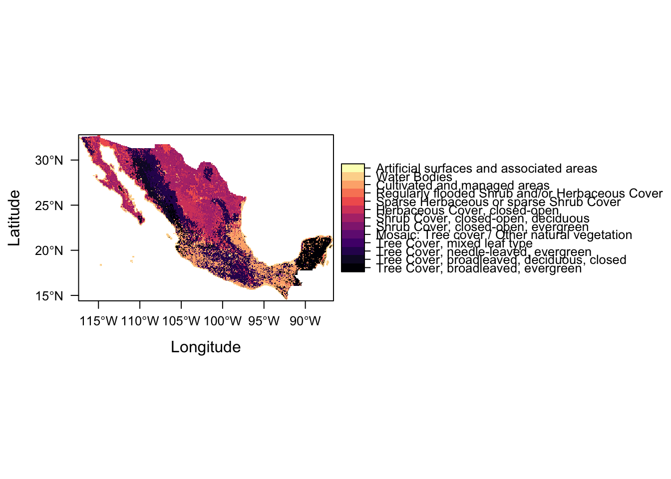
Expand here to see past versions of unnamed-chunk-25-1.png:</em></summary>
<table style="border-collapse:separate; border-spacing:5px;">
<thead>
<tr>
<th style="text-align:left;">
Version
</th>
<th style="text-align:left;">
Author
</th>
<th style="text-align:left;">
Date
</th>
</tr>
</thead>
<tbody>
<tr>
<td style="text-align:left;">
<a href="https://github.com/annakrystalli/intro-r-gis/blob/f94df5ce59f87379087af9763c9e1b64f7e9c0f3/docs/figure/raster.Rmd/unnamed-chunk-25-1.png" target="_blank">f94df5c</a>
</td>
<td style="text-align:left;">
annakrystalli
</td>
<td style="text-align:left;">
2018-09-04
</td>
</tr>
</tbody>
</table>
<p></details></p>
<p>Success!</p>
<p>And seeing as we’re dealing with primarily vegetation, let’s create a new map theme (colour palette) using function <code>rasterVis::rasterTheme</code> and <a href="http://colorbrewer2.org/#type=sequential&amp;scheme=YlGn&amp;n=9">colour brewer palette Yellow &amp; Greens (“YlGn”)</a>.</p>
<div class="sourceCode"><pre class="sourceCode r"><code class="sourceCode r">mapTheme &lt;-<span class="st"> </span><span class="kw">rasterTheme</span>(<span class="dt">region =</span> <span class="kw">rev</span>(<span class="kw">brewer.pal</span>(<span class="dv">9</span>,<span class="st">&quot;YlGn&quot;</span>)))
<span class="kw">levelplot</span>(lc, <span class="dt">par.settings =</span> mapTheme)</code></pre></div>
<p><img src="figure/raster.Rmd/unnamed-chunk-26-1.png" width="672" style="display: block; margin: auto;" /></p>
<details> <summary><em>
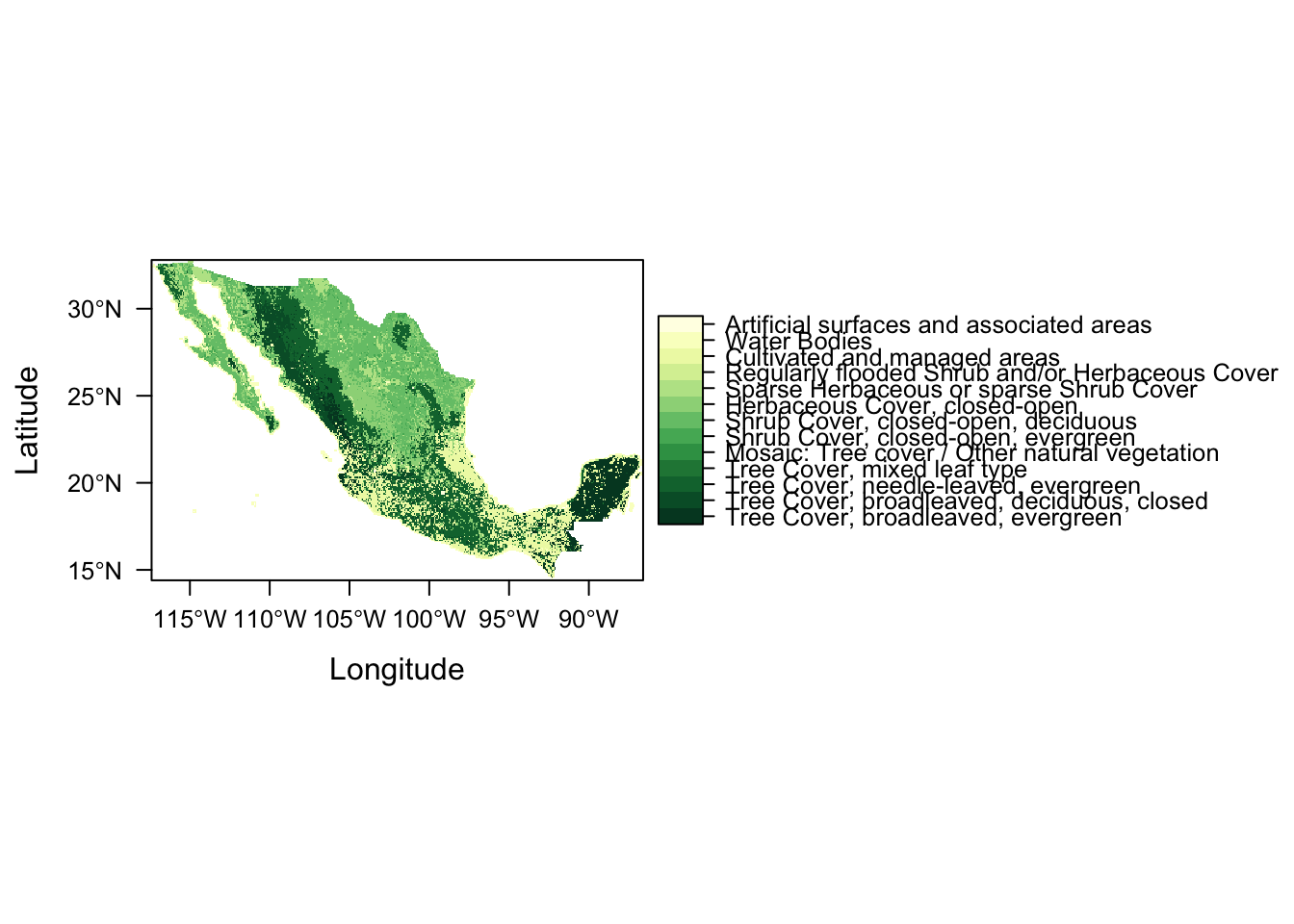
Expand here to see past versions of unnamed-chunk-26-1.png:</em></summary>
<table style="border-collapse:separate; border-spacing:5px;">
<thead>
<tr>
<th style="text-align:left;">
Version
</th>
<th style="text-align:left;">
Author
</th>
<th style="text-align:left;">
Date
</th>
</tr>
</thead>
<tbody>
<tr>
<td style="text-align:left;">
<a href="https://github.com/annakrystalli/intro-r-gis/blob/f94df5ce59f87379087af9763c9e1b64f7e9c0f3/docs/figure/raster.Rmd/unnamed-chunk-26-1.png" target="_blank">f94df5c</a>
</td>
<td style="text-align:left;">
annakrystalli
</td>
<td style="text-align:left;">
2018-09-04
</td>
</tr>
</tbody>
</table>
<p></details></p>
<p>The function takes a vector of colours to produce a colour gradient that is then mapped to raster values. It has a numer of in-built colour vectors to choose from and you can even provide your own custom vectors of functions (which is what we would probably want to do in our case to make the colour more reflective of the vegetation type).</p>
</div>
</div>
<div id="stacking-rasterlayers" class="section level2">
<h2>stacking <code>rasterLayers</code></h2>
<div class="sourceCode"><pre class="sourceCode r"><code class="sourceCode r"><span class="kw">stack</span>(st, lc)</code></pre></div>
<pre><code>Error in compareRaster(x): different extent</code></pre>
<p>This doesn’t work, notifying us that there is a problem with mismatching extents. We don’t really need the whole extent of data anyways so let’s try croping everything to the same extent, that of the study area bounding box we defined in our vector workflow</p>
<p>So let’s load the molecular data that we have converted to an <code>sf</code> using function <code>sf::read_sf</code> and recreate a bounding box.</p>
<div class="sourceCode"><pre class="sourceCode r"><code class="sourceCode r">mol_sf &lt;-<span class="st"> </span><span class="kw">read_sf</span>(here<span class="op">::</span><span class="kw">here</span>(<span class="st">&quot;data&quot;</span>, <span class="st">&quot;sf&quot;</span>, <span class="st">&quot;salamander.geojson&quot;</span>))
study_bbox &lt;-<span class="st"> </span>mol_sf <span class="op">%&gt;%</span><span class="st"> </span><span class="kw">st_bbox</span>() <span class="op">%&gt;%</span><span class="st"> </span><span class="kw">st_as_sfc</span>()</code></pre></div>
<p>This bounding box is really tight around our data points. To ensure our raster data contain the locations of all our data points, let’s give this extraction bounding box some space around our points using function <code>sf::st_buffer</code>.</p>
<p><em>Looking at the help file for this function using <code>?st_buffer</code> gives us information on a whole suite of useful functions to perform geometric operations on simple feature geometry sets.</em></p>
<div class="sourceCode"><pre class="sourceCode r"><code class="sourceCode r">extract_bbox &lt;-<span class="st"> </span>study_bbox <span class="op">%&gt;%</span><span class="st"> </span><span class="kw">st_buffer</span>(<span class="dt">dist =</span> <span class="dv">1</span>)</code></pre></div>
<pre><code>Warning in st_buffer.sfc(., dist = 1): st_buffer does not correctly buffer
longitude/latitude data</code></pre>
<div class="sourceCode"><pre class="sourceCode r"><code class="sourceCode r">extract_bbox</code></pre></div>
<pre><code>Geometry set for 1 feature 
geometry type:  POLYGON
dimension:      XY
bbox:           xmin: -100.8481 ymin: 17.94194 xmax: -96.09056 ymax: 20.63083
epsg (SRID):    4326
proj4string:    +proj=longlat +datum=WGS84 +no_defs</code></pre>
<p>To crop a raster we use function <code>raster::crop</code> which will returns a geographic subset of the raster as specified either by an <code>Extent</code> object or an object from which an extent object can be extracted/created.</p>
<p>In our case, we’ll use the <code>extract_bbox</code> <code>sf</code> we just created. So let’s try and crop <code>lc</code> first.</p>
<div class="sourceCode"><pre class="sourceCode r"><code class="sourceCode r"><span class="kw">crop</span>(lc, extract_bbox)</code></pre></div>
<pre><code>Error in .local(x, y, ...): Cannot get an Extent object from argument y</code></pre>
<p>Ooops! That throws an error! That’s because of current <code>sf</code> and <code>raster</code> compatibility issues. All we need to do though is convert our <code>sf</code> to an <code>sp</code> spatial class object which <code>raster</code> is designed to work with. We can do this with function <code>sf::as_Spatial</code>.</p>
<div class="sourceCode"><pre class="sourceCode r"><code class="sourceCode r">sp_extract_bbox &lt;-<span class="st"> </span><span class="kw">as_Spatial</span>(extract_bbox)
sp_extract_bbox</code></pre></div>
<pre><code>class       : SpatialPolygons 
features    : 1 
extent      : -100.8481, -96.09056, 17.94194, 20.63083  (xmin, xmax, ymin, ymax)
coord. ref. : +proj=longlat +datum=WGS84 +no_defs +ellps=WGS84 +towgs84=0,0,0 </code></pre>
<p>Let’s try now.</p>
<div class="sourceCode"><pre class="sourceCode r"><code class="sourceCode r"><span class="kw">crop</span>(lc, sp_extract_bbox)</code></pre></div>
<pre><code>class       : RasterLayer 
dimensions  : 323, 571, 184433  (nrow, ncol, ncell)
resolution  : 0.008333333, 0.008333333  (x, y)
extent      : -100.85, -96.09167, 17.94167, 20.63333  (xmin, xmax, ymin, ymax)
coord. ref. : +proj=longlat +ellps=WGS84 
data source : in memory
names       : MEX_msk_cov 
values      : 1, 22  (min, max)
attributes  :
       ID                                    descr
 from:  1       Tree Cover, broadleaved, evergreen
 to  : 22 Artificial surfaces and associated areas</code></pre>
<p>Success! This works.</p>
<p>So let’s stack and crop all in one go:</p>
<div class="sourceCode"><pre class="sourceCode r"><code class="sourceCode r">full_stack &lt;-<span class="st"> </span><span class="kw">stack</span>(
<span class="kw">crop</span>(lc, sp_extract_bbox),
<span class="kw">crop</span>(st, sp_extract_bbox)
)

full_stack</code></pre></div>
<pre><code>class       : RasterStack 
dimensions  : 323, 571, 184433, 5  (nrow, ncol, ncell, nlayers)
resolution  : 0.008333333, 0.008333333  (x, y)
extent      : -100.85, -96.09167, 17.94167, 20.63333  (xmin, xmax, ymin, ymax)
coord. ref. : +proj=longlat +ellps=WGS84 
names       : MEX_msk_cov, mx.bio_15, mx.bio_4, mx.bio_5, mx.bio_6 
min values  :           1,        41,      655,       54,      -83 
max values  :          22,       117,     3387,      411,      180 </code></pre>
<p>Awesome! We’ve now got all our initial raster files in a single <code>rasterStack</code> 🎉. We’re not done though. There are two things we need to address for our final <code>rasterStack</code>.</p>
<ol style="list-style-type: decimal">
<li>We want the <strong>temperature range</strong> (ie the difference between <code>mx.bio_5</code> and <code>mx.bio_6</code>) for our SDM rather than the extremes.</li>
<li>We also still need to address the fact that our <strong>temperature data is currrently in degrees C x 10</strong>.</li>
</ol>
<p>So let’s try and address this by creating a new <code>rasterStack</code> from the layers in our <code>full_stack</code>. We use function <code>raster::stack()</code> again.</p>
<div class="sourceCode"><pre class="sourceCode r"><code class="sourceCode r">env_stack &lt;-<span class="st"> </span><span class="kw">stack</span>(
    (full_stack[[<span class="st">&quot;mx.bio_5&quot;</span>]] <span class="op">-</span><span class="st"> </span>full_stack[[<span class="st">&quot;mx.bio_6&quot;</span>]])<span class="op">/</span><span class="dv">10</span>,
    full_stack[[<span class="st">&quot;mx.bio_4&quot;</span>]], 
    full_stack[[<span class="st">&quot;mx.bio_15&quot;</span>]],
    full_stack[[<span class="st">&quot;MEX_msk_cov&quot;</span>]])

env_stack</code></pre></div>
<pre><code>class       : RasterStack 
dimensions  : 323, 571, 184433, 4  (nrow, ncol, ncell, nlayers)
resolution  : 0.008333333, 0.008333333  (x, y)
extent      : -100.85, -96.09167, 17.94167, 20.63333  (xmin, xmax, ymin, ymax)
coord. ref. : +proj=longlat +datum=WGS84 +no_defs +ellps=WGS84 +towgs84=0,0,0 
names       :  layer, mx.bio_4, mx.bio_15, MEX_msk_cov 
min values  :   13.7,    655.0,      41.0,         1.0 
max values  :   27.2,   3387.0,     117.0,        22.0 </code></pre>
<p>Let’s give our layers better names. This is easily achieved with function <code>names()</code></p>
<div class="sourceCode"><pre class="sourceCode r"><code class="sourceCode r"><span class="kw">names</span>(env_stack) &lt;-<span class="st"> </span><span class="kw">c</span>(<span class="st">&quot;temp_range&quot;</span>,<span class="st">&quot;temp_seasonality&quot;</span>, 
                     <span class="st">&quot;prec_seasonality&quot;</span>, <span class="st">&quot;land_cover&quot;</span>)
env_stack</code></pre></div>
<pre><code>class       : RasterStack 
dimensions  : 323, 571, 184433, 4  (nrow, ncol, ncell, nlayers)
resolution  : 0.008333333, 0.008333333  (x, y)
extent      : -100.85, -96.09167, 17.94167, 20.63333  (xmin, xmax, ymin, ymax)
coord. ref. : +proj=longlat +datum=WGS84 +no_defs +ellps=WGS84 +towgs84=0,0,0 
names       : temp_range, temp_seasonality, prec_seasonality, land_cover 
min values  :       13.7,            655.0,             41.0,        1.0 
max values  :       27.2,           3387.0,            117.0,       22.0 </code></pre>
<div id="exercise" class="section level3">
<h3>Exercise</h3>
<div id="create-and-plot-a-new-rasterlayer-of-rough-mean-temperature." class="section level4">
<h4><strong>1) Create and plot a new <code>rasterLayer</code> of rough mean temperature.</strong></h4>
<p>(rough because it would be much better to use more data at higher temporal resolution, eg at least monthly, not extremes).</p>
</div>
</div>
<div id="plotting-our-rasterstack" class="section level3">
<h3>plotting our <code>rasterStack</code></h3>
<p>Let’s try and plot our new environmental stack.</p>
<div class="sourceCode"><pre class="sourceCode r"><code class="sourceCode r"><span class="kw">levelplot</span>(env_stack)</code></pre></div>
<pre><code>Error in .checkLevels(levs[[j]], value[[j]]): new raster attributes (factor values) should be in a data.frame (inside a list)</code></pre>
<p>This doesn’t work now because we are trying to mix displaying factor and numeric data.</p>
<p>We can still extract and plot individual layers though.</p>
<div class="sourceCode"><pre class="sourceCode r"><code class="sourceCode r"><span class="kw">levelplot</span>(env_stack, <span class="dt">layers =</span> <span class="st">&quot;temp_seasonality&quot;</span>)</code></pre></div>
<p><img src="figure/raster.Rmd/unnamed-chunk-37-1.png" width="672" style="display: block; margin: auto;" /></p>
<details> <summary><em>
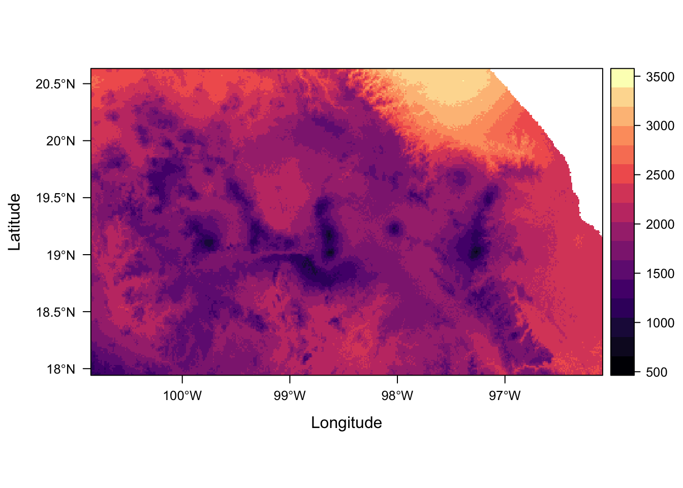
Expand here to see past versions of unnamed-chunk-37-1.png:</em></summary>
<table style="border-collapse:separate; border-spacing:5px;">
<thead>
<tr>
<th style="text-align:left;">
Version
</th>
<th style="text-align:left;">
Author
</th>
<th style="text-align:left;">
Date
</th>
</tr>
</thead>
<tbody>
<tr>
<td style="text-align:left;">
<a href="https://github.com/annakrystalli/intro-r-gis/blob/f94df5ce59f87379087af9763c9e1b64f7e9c0f3/docs/figure/raster.Rmd/unnamed-chunk-37-1.png" target="_blank">f94df5c</a>
</td>
<td style="text-align:left;">
annakrystalli
</td>
<td style="text-align:left;">
2018-09-04
</td>
</tr>
</tbody>
</table>
<p></details></p>
<p>For more details on how to plot several <code>rasterLayers</code> with different legends (including different data types) in the <code>rasterVis</code> package <a href="https://oscarperpinan.github.io/rastervis/FAQ.html#several_rasters">FAQs</a>. It would also solve the problem we had earlier with plotting multiple layers using the same scale.</p>
</div>
</div>
</div>
<div id="saving-raster-data" class="section level1">
<h1>Saving raster data</h1>
<p>A number of drivers are available to write raster data to a number of gridded geospatial file types:</p>
<div class="sourceCode"><pre class="sourceCode r"><code class="sourceCode r">raster<span class="op">::</span><span class="kw">writeFormats</span>() <span class="op">%&gt;%</span><span class="st"> </span>knitr<span class="op">::</span><span class="kw">kable</span>()</code></pre></div>
<table>
<thead>
<tr class="header">
<th align="left">name</th>
<th align="left">long_name</th>
</tr>
</thead>
<tbody>
<tr class="odd">
<td align="left">raster</td>
<td align="left">R-raster</td>
</tr>
<tr class="even">
<td align="left">SAGA</td>
<td align="left">SAGA GIS</td>
</tr>
<tr class="odd">
<td align="left">IDRISI</td>
</tr>
<tr class="even">
<td align="left">IDRISIold</td>
<td align="left">IDRISI (img/doc)</td>
</tr>
<tr class="odd">
<td align="left">BIL</td>
<td align="left">Band by Line</td>
</tr>
<tr class="even">
<td align="left">BSQ</td>
<td align="left">Band Sequential</td>
</tr>
<tr class="odd">
<td align="left">BIP</td>
<td align="left">Band by Pixel</td>
</tr>
<tr class="even">
<td align="left">ascii</td>
<td align="left">Arc ASCII</td>
</tr>
<tr class="odd">
<td align="left">CDF</td>
<td align="left">NetCDF</td>
</tr>
<tr class="even">
<td align="left">big</td>
<td align="left">big.matrix</td>
</tr>
<tr class="odd">
<td align="left">ADRG</td>
<td align="left">ARC Digitized Raster Graphics</td>
</tr>
<tr class="even">
<td align="left">BMP</td>
<td align="left">MS Windows Device Independent Bitmap</td>
</tr>
<tr class="odd">
<td align="left">BT</td>
<td align="left">VTP .bt (Binary Terrain) 1.3 Format</td>
</tr>
<tr class="even">
<td align="left">CTable2</td>
<td align="left">CTable2 Datum Grid Shift</td>
</tr>
<tr class="odd">
<td align="left">EHdr</td>
<td align="left">ESRI .hdr Labelled</td>
</tr>
<tr class="even">
<td align="left">ELAS</td>
</tr>
<tr class="odd">
<td align="left">ENVI</td>
<td align="left">ENVI .hdr Labelled</td>
</tr>
<tr class="even">
<td align="left">ERS</td>
<td align="left">ERMapper .ers Labelled</td>
</tr>
<tr class="odd">
<td align="left">GPKG</td>
<td align="left">GeoPackage</td>
</tr>
<tr class="even">
<td align="left">GS7BG</td>
<td align="left">Golden Software 7 Binary Grid (.grd)</td>
</tr>
<tr class="odd">
<td align="left">GSBG</td>
<td align="left">Golden Software Binary Grid (.grd)</td>
</tr>
<tr class="even">
<td align="left">GTiff</td>
<td align="left">GeoTIFF</td>
</tr>
<tr class="odd">
<td align="left">GTX</td>
<td align="left">NOAA Vertical Datum .GTX</td>
</tr>
<tr class="even">
<td align="left">HFA</td>
<td align="left">Erdas Imagine Images (.img)</td>
</tr>
<tr class="odd">
<td align="left">IDA</td>
<td align="left">Image Data and Analysis</td>
</tr>
<tr class="even">
<td align="left">ILWIS</td>
<td align="left">ILWIS Raster Map</td>
</tr>
<tr class="odd">
<td align="left">INGR</td>
<td align="left">Intergraph Raster</td>
</tr>
<tr class="even">
<td align="left">ISCE</td>
<td align="left">ISCE raster</td>
</tr>
<tr class="odd">
<td align="left">ISIS2</td>
<td align="left">USGS Astrogeology ISIS cube (Version 2)</td>
</tr>
<tr class="even">
<td align="left">KRO</td>
<td align="left">KOLOR Raw</td>
</tr>
<tr class="odd">
<td align="left">LAN</td>
<td align="left">Erdas .LAN/.GIS</td>
</tr>
<tr class="even">
<td align="left">Leveller</td>
<td align="left">Leveller heightfield</td>
</tr>
<tr class="odd">
<td align="left">MBTiles</td>
</tr>
<tr class="even">
<td align="left">MRF</td>
<td align="left">Meta Raster Format</td>
</tr>
<tr class="odd">
<td align="left">netCDF</td>
<td align="left">Network Common Data Format</td>
</tr>
<tr class="even">
<td align="left">NITF</td>
<td align="left">National Imagery Transmission Format</td>
</tr>
<tr class="odd">
<td align="left">NTv2</td>
<td align="left">NTv2 Datum Grid Shift</td>
</tr>
<tr class="even">
<td align="left">PAux</td>
<td align="left">PCI .aux Labelled</td>
</tr>
<tr class="odd">
<td align="left">PCIDSK</td>
<td align="left">PCIDSK Database File</td>
</tr>
<tr class="even">
<td align="left">PCRaster</td>
<td align="left">PCRaster Raster File</td>
</tr>
<tr class="odd">
<td align="left">PDF</td>
<td align="left">Geospatial PDF</td>
</tr>
<tr class="even">
<td align="left">PNM</td>
<td align="left">Portable Pixmap Format (netpbm)</td>
</tr>
<tr class="odd">
<td align="left">RMF</td>
<td align="left">Raster Matrix Format</td>
</tr>
<tr class="even">
<td align="left">ROI_PAC</td>
<td align="left">ROI_PAC raster</td>
</tr>
<tr class="odd">
<td align="left">RST</td>
<td align="left">Idrisi Raster A.1</td>
</tr>
<tr class="even">
<td align="left">SAGA</td>
<td align="left">SAGA GIS Binary Grid (.sdat)</td>
</tr>
<tr class="odd">
<td align="left">SGI</td>
<td align="left">SGI Image File Format 1.0</td>
</tr>
<tr class="even">
<td align="left">Terragen</td>
<td align="left">Terragen heightfield</td>
</tr>
</tbody>
</table>
<div id="save-rasterstack" class="section level3">
<h3>Save <code>rasterStack</code></h3>
<p>So let’s finally save our raster stack as a binary ‘Native’ <code>raster</code> package <code>.grd</code> file format using function <code>raster::writeRaster()</code>. We’ll do that to preserve the layer names in the <code>rasterStack</code>. It also allows us to combine categorical and numeric layers in one file.</p>
<div class="sourceCode"><pre class="sourceCode r"><code class="sourceCode r"><span class="kw">writeRaster</span>(env_stack, <span class="dt">filename =</span> here<span class="op">::</span><span class="kw">here</span>(<span class="st">&quot;data&quot;</span>, <span class="st">&quot;raster&quot;</span>, <span class="st">&quot;env_stack.grd&quot;</span>))</code></pre></div>
<p>However, these files are not compressed. If the size of the files is an issue, we can save each file as an individual GeoTiff file and reimport them all together into a stack later on.</p>
<div class="sourceCode"><pre class="sourceCode r"><code class="sourceCode r"><span class="kw">dir.create</span>(here<span class="op">::</span><span class="kw">here</span>(<span class="st">&quot;data&quot;</span>, <span class="st">&quot;raster&quot;</span>, <span class="st">&quot;processed&quot;</span>))

<span class="kw">writeRaster</span>(env_stack, 
            <span class="dt">filename=</span>here<span class="op">::</span><span class="kw">here</span>(<span class="st">&quot;data&quot;</span>, <span class="st">&quot;raster&quot;</span> , 
                                <span class="st">&quot;processed&quot;</span>, <span class="st">&quot;env_stack.tif&quot;</span>),
            <span class="dt">bylayer =</span> T, <span class="dt">suffix =</span> <span class="kw">names</span>(env_stack))</code></pre></div>
<p>The following code lists all the files in the <code>processed</code> folder, matching only those files that end with <code>.tiff</code> (ignoring the <code>env_land_cover.tif.aux.xml</code> file which contains the RAT and would throw an error), reads and stacks them!</p>
<div class="sourceCode"><pre class="sourceCode r"><code class="sourceCode r"><span class="kw">stack</span>(<span class="kw">list.files</span>(here<span class="op">::</span><span class="kw">here</span>(<span class="st">&quot;data&quot;</span>, <span class="st">&quot;raster&quot;</span> , <span class="st">&quot;processed&quot;</span>),
                 <span class="dt">pattern =</span> <span class="st">&quot;.tif$&quot;</span>,
                 <span class="dt">full.names =</span> T))</code></pre></div>
<pre><code>class       : RasterStack 
dimensions  : 323, 571, 184433, 4  (nrow, ncol, ncell, nlayers)
resolution  : 0.008333333, 0.008333333  (x, y)
extent      : -100.85, -96.09167, 17.94167, 20.63333  (xmin, xmax, ymin, ymax)
coord. ref. : +proj=longlat +ellps=WGS84 +no_defs 
names       : env_stack_land_cover, env_stack_prec_seasonality, env_stack_temp_range, env_stack_temp_seasonality 
min values  :                  1.0,                       41.0,                 13.7,                      655.0 
max values  :                 22.0,                      117.0,                 27.2,                     3387.0 </code></pre>
</div>
</div>
<div id="extracting-and-summarising-raster-data" class="section level1">
<h1>Extracting and summarising raster data</h1>
<div id="extracting-points" class="section level3">
<h3>extracting points</h3>
<p>We can extract data underlying an <code>sf</code> from a raster using function <code>raster::extract()</code>. The output in the case of points is a single value for each point. This is returned as a vector for a single layer or a matrix for multiple layers, as is our case.</p>
<p>Let’s have a look at our data again</p>
<div class="sourceCode"><pre class="sourceCode r"><code class="sourceCode r">mol_sf</code></pre></div>
<pre><code>Simple feature collection with 15 features and 9 fields
geometry type:  POINT
dimension:      XY
bbox:           xmin: -99.84806 ymin: 18.94194 xmax: -97.09056 ymax: 19.63083
epsg (SRID):    4326
proj4string:    +proj=longlat +datum=WGS84 +no_defs
# A tibble: 15 x 10
      id locality       n mountain_chain   region    na    he    ar    par
   &lt;int&gt; &lt;chr&gt;      &lt;int&gt; &lt;chr&gt;            &lt;chr&gt;  &lt;dbl&gt; &lt;dbl&gt; &lt;dbl&gt;  &lt;dbl&gt;
 1     1 Nevado de…    12 Nevado de Toluca Centr…  5.44 0.620  4.56 0.350 
 2     2 Texcalyac…    29 Sierra de las C… Centr…  8.22 0.660  5.14 0.500 
 3     3 Desierto …     7 Sierra de las C… Centr…  4.44 0.590  4.44 0.180 
 4     4 Ajusco         8 Sierra de las C… Centr…  4.22 0.490  4.05 0.0200
 5     8 Calpan        34 Sierra Nevada    Centr… 11.9  0.730  6.48 0.290 
 6     9 Atzompa       43 Sierra Nevada    Centr… 10.3  0.690  5.79 0.0800
 7    10 Llano Gra…    15 Sierra Nevada (… Centr…  7.78 0.650  5.80 0.250 
 8    11 Rio Frio      27 Sierra Nevada (… Centr…  7.56 0.570  4.77 0.130 
 9    12 Nanacamil…    14 Sierra Nevada (… Centr…  6.22 0.590  4.91 0.100 
10    13 MalincheS      8 Malinche         Centr…  5.00 0.580  4.69 0.0900
11    14 MalincheW     17 Malinche         Centr…  6.67 0.600  4.76 0.0600
12    16 MalincheE     13 Malinche         Centr…  6.11 0.560  4.73 0.210 
13    17 Texmalaqu…     8 Pico de Orizaba  South…  6.00 0.710  5.64 0.910 
14    18 Xometla       16 Pico de Orizaba  South…  9.11 0.830  6.86 0.490 
15    19 Vigas         48 Cofre de Perote  North… 11.8  0.660  5.75 1.31  
# ... with 1 more variable: geometry &lt;POINT [°]&gt;</code></pre>
<p>Because we want to combine it with our previous data in <code>mol_sf</code> we’ll pipe the resulting matrix into <code>as.data.frame</code> so we can easily bind our extracted environmental data to our molecular data.</p>
<div class="sourceCode"><pre class="sourceCode r"><code class="sourceCode r">env_points &lt;-<span class="st"> </span><span class="kw">extract</span>(env_stack, <span class="kw">as_Spatial</span>(mol_sf)) <span class="op">%&gt;%</span><span class="st"> </span><span class="kw">as.data.frame</span>()

mol_env_sf &lt;-<span class="st"> </span><span class="kw">bind_cols</span>(mol_sf, env_points)
mol_env_sf</code></pre></div>
<pre><code>Simple feature collection with 15 features and 13 fields
geometry type:  POINT
dimension:      XY
bbox:           xmin: -99.84806 ymin: 18.94194 xmax: -97.09056 ymax: 19.63083
epsg (SRID):    4326
proj4string:    +proj=longlat +datum=WGS84 +no_defs
# A tibble: 15 x 14
      id locality       n mountain_chain   region    na    he    ar    par
   &lt;int&gt; &lt;chr&gt;      &lt;int&gt; &lt;chr&gt;            &lt;chr&gt;  &lt;dbl&gt; &lt;dbl&gt; &lt;dbl&gt;  &lt;dbl&gt;
 1     1 Nevado de…    12 Nevado de Toluca Centr…  5.44 0.620  4.56 0.350 
 2     2 Texcalyac…    29 Sierra de las C… Centr…  8.22 0.660  5.14 0.500 
 3     3 Desierto …     7 Sierra de las C… Centr…  4.44 0.590  4.44 0.180 
 4     4 Ajusco         8 Sierra de las C… Centr…  4.22 0.490  4.05 0.0200
 5     8 Calpan        34 Sierra Nevada    Centr… 11.9  0.730  6.48 0.290 
 6     9 Atzompa       43 Sierra Nevada    Centr… 10.3  0.690  5.79 0.0800
 7    10 Llano Gra…    15 Sierra Nevada (… Centr…  7.78 0.650  5.80 0.250 
 8    11 Rio Frio      27 Sierra Nevada (… Centr…  7.56 0.570  4.77 0.130 
 9    12 Nanacamil…    14 Sierra Nevada (… Centr…  6.22 0.590  4.91 0.100 
10    13 MalincheS      8 Malinche         Centr…  5.00 0.580  4.69 0.0900
11    14 MalincheW     17 Malinche         Centr…  6.67 0.600  4.76 0.0600
12    16 MalincheE     13 Malinche         Centr…  6.11 0.560  4.73 0.210 
13    17 Texmalaqu…     8 Pico de Orizaba  South…  6.00 0.710  5.64 0.910 
14    18 Xometla       16 Pico de Orizaba  South…  9.11 0.830  6.86 0.490 
15    19 Vigas         48 Cofre de Perote  North… 11.8  0.660  5.75 1.31  
# ... with 5 more variables: geometry &lt;POINT [°]&gt;, temp_range &lt;dbl&gt;,
#   temp_seasonality &lt;dbl&gt;, prec_seasonality &lt;dbl&gt;, land_cover &lt;dbl&gt;</code></pre>
<p>Our new <code>sf</code> is now ready to use for species distribution modelling. But we can also start visualising the relationships between our molecular and environmental variables</p>
<div class="sourceCode"><pre class="sourceCode r"><code class="sourceCode r"><span class="kw">ggplot</span>(mol_env_sf, <span class="kw">aes</span>(<span class="dt">x =</span> temp_range, <span class="dt">y =</span> na, <span class="dt">colour =</span> region)) <span class="op">+</span>
<span class="st">    </span><span class="kw">geom_point</span>()</code></pre></div>
<p><img src="figure/raster.Rmd/unnamed-chunk-44-1.png" width="672" style="display: block; margin: auto;" /></p>
<details> <summary><em>
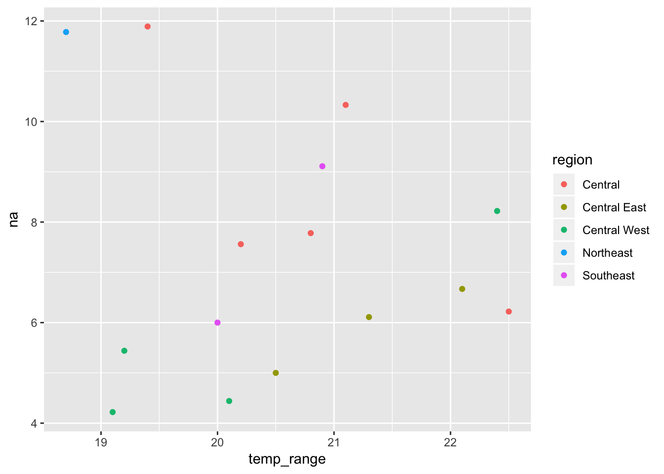
Expand here to see past versions of unnamed-chunk-44-1.png:</em></summary>
<table style="border-collapse:separate; border-spacing:5px;">
<thead>
<tr>
<th style="text-align:left;">
Version
</th>
<th style="text-align:left;">
Author
</th>
<th style="text-align:left;">
Date
</th>
</tr>
</thead>
<tbody>
<tr>
<td style="text-align:left;">
<a href="https://github.com/annakrystalli/intro-r-gis/blob/c91966eb061c8c7b7d8dbec843e427d1d673013d/docs/figure/raster.Rmd/unnamed-chunk-44-1.png" target="_blank">c91966e</a>
</td>
<td style="text-align:left;">
annakrystalli
</td>
<td style="text-align:left;">
2018-09-05
</td>
</tr>
</tbody>
</table>
<p></details></p>
</div>
<div id="extracting-and-summarising-raster-data-using-polygons" class="section level3">
<h3>extracting and summarising raster data using polygons</h3>
<p>We can also extract and summarise data over an area represented by a polygon using using the <code>raster::extract()</code> function. If we want a summarising function to be applied to the pixel values returned by the extraction, we can supply it to argument <code>fun</code>. Let’s calculate the <strong>mean <code>temp_range</code> across the <code>study_bbox</code> area</strong>.</p>
<div class="sourceCode"><pre class="sourceCode r"><code class="sourceCode r">mean_temp_range &lt;-<span class="st"> </span><span class="kw">extract</span>(env_stack[[<span class="st">&quot;temp_range&quot;</span>]], 
                <span class="kw">as_Spatial</span>(study_bbox),
                <span class="dt">fun =</span> mean,
                <span class="dt">na.rm =</span> T)

mean_temp_range</code></pre></div>
<pre><code>         [,1]
[1,] 22.21228</code></pre>
<p>Let’s use this to calculate the deviation of each of our data points from the study box mean we just calculated. We can use <code>dplyr::mutate</code> to manipulate attribute data in our <code>sf</code> just like any other data.frame.</p>
<div class="sourceCode"><pre class="sourceCode r"><code class="sourceCode r">mol_env_sf &lt;-<span class="st"> </span>mol_env_sf <span class="op">%&gt;%</span><span class="st"> </span>
<span class="st">    </span><span class="kw">mutate</span>(<span class="dt">dev_temp_range =</span> temp_range <span class="op">-</span><span class="st"> </span><span class="kw">as.vector</span>(mean_temp_range))</code></pre></div>
<div class="sourceCode"><pre class="sourceCode r"><code class="sourceCode r">mol_env_sf <span class="op">%&gt;%</span><span class="st"> </span><span class="kw">select</span>(locality, dev_temp_range)</code></pre></div>
<pre><code>Simple feature collection with 15 features and 2 fields
geometry type:  POINT
dimension:      XY
bbox:           xmin: -99.84806 ymin: 18.94194 xmax: -97.09056 ymax: 19.63083
epsg (SRID):    4326
proj4string:    +proj=longlat +datum=WGS84 +no_defs
# A tibble: 15 x 3
   locality               dev_temp_range             geometry
   &lt;chr&gt;                           &lt;dbl&gt;          &lt;POINT [°]&gt;
 1 Nevado de Toluca               -3.01  (-99.84806 19.19361)
 2 Texcalyacac                     0.188     (-99.5 19.12056)
 3 Desierto de los Leones         -2.11  (-99.30056 19.26667)
 4 Ajusco                         -3.11      (-99.3 19.18278)
 5 Calpan                         -2.81  (-98.59167 19.13139)
 6 Atzompa                        -1.11  (-98.55972 19.18056)
 7 Llano Grande                   -1.41  (-98.72056 19.33889)
 8 Rio Frio                       -2.01  (-98.69472 19.36611)
 9 Nanacamilpa                     0.288 (-98.59611 19.48028)
10 MalincheS                      -1.71  (-98.02194 19.18722)
11 MalincheW                      -0.112   (-98.095 19.25778)
12 MalincheE                      -0.912      (-97.975 19.23)
13 Texmalaquilla                  -2.21     (-97.29 18.94194)
14 Xometla                        -1.31    (-97.19056 18.975)
15 Vigas                          -3.51  (-97.09056 19.63083)</code></pre>
<p>Let’s save our final <code>sf</code> now containing the environmental data we extracted</p>
<div class="sourceCode"><pre class="sourceCode r"><code class="sourceCode r"><span class="kw">write_sf</span>(mol_env_sf, here<span class="op">::</span><span class="kw">here</span>(<span class="st">&quot;data&quot;</span>, <span class="st">&quot;sf&quot;</span>, <span class="st">&quot;env_salamander.geojson&quot;</span>))</code></pre></div>
</div>
<div id="exercise-1" class="section level3">
<h3>Exercise</h3>
<div id="calculate-mean-precipitation-seasonality-for-the-extraction-bounding-box-area.-what-is-the-value" class="section level4">
<h4>2) Calculate mean precipitation seasonality for the <strong>extraction bounding box area</strong>. What is the value?</h4>
</div>
<div id="add-a-column-indicating-whether-data-points-are-greater-than-true-or-less-than-false-extraction-area-mean-precipitation-seasonality." class="section level4">
<h4>3) Add a column indicating whether data points are greater than (<code>TRUE</code>) or less than (<code>FALSE</code>) extraction area mean precipitation seasonality.</h4>
<p><br></p>
<hr />
</div>
</div>
<div id="other-useful-raster-functions-you-should-know-about" class="section level3">
<h3>Other useful <code>raster</code> functions you should know about:</h3>
<p><a href="http://rspatial.org/spatial/rst/8-rastermanip.html" class="uri">http://rspatial.org/spatial/rst/8-rastermanip.html</a></p>
<ul>
<li><code>merge</code>: merge <code>rasterLayers</code></li>
<li><code>trim</code>: remove outer <code>NA</code> rows and columns</li>
<li><code>extend</code>: expand margins with <code>NA</code>.</li>
<li><code>projectRaster</code>: Project the values of a Raster* object to a new Raster* object with another projection (coordinate reference system, (CRS)).</li>
</ul>
</div>
<div id="session-information" class="section level2">
<h2>Session information</h2>
<div class="sourceCode"><pre class="sourceCode r"><code class="sourceCode r"><span class="kw">sessionInfo</span>()</code></pre></div>
<pre><code>R version 3.4.4 (2018-03-15)
Platform: x86_64-apple-darwin15.6.0 (64-bit)
Running under: macOS High Sierra 10.13.3

Matrix products: default
BLAS: /Library/Frameworks/R.framework/Versions/3.4/Resources/lib/libRblas.0.dylib
LAPACK: /Library/Frameworks/R.framework/Versions/3.4/Resources/lib/libRlapack.dylib

locale:
[1] en_GB.UTF-8/en_GB.UTF-8/en_GB.UTF-8/C/en_GB.UTF-8/en_GB.UTF-8

attached base packages:
[1] stats     graphics  grDevices utils     datasets  methods   base     

other attached packages:
 [1] bindrcpp_0.2.2      ggplot2_3.0.0       dplyr_0.7.6        
 [4] sf_0.6-3            rasterVis_0.45      latticeExtra_0.6-28
 [7] RColorBrewer_1.1-2  lattice_0.20-35     raster_2.6-7       
[10] sp_1.2-5           

loaded via a namespace (and not attached):
 [1] zoo_1.8-3         tidyselect_0.2.4  purrr_0.2.5      
 [4] colorspace_1.3-2  htmltools_0.3.6   viridisLite_0.3.0
 [7] emo_0.0.0.9000    yaml_2.1.19       utf8_1.1.3       
[10] rlang_0.2.1       R.oo_1.21.0       e1071_1.6-8      
[13] hexbin_1.27.1     pillar_1.2.1      glue_1.2.0.9000  
[16] withr_2.1.2       DBI_1.0.0         R.utils_2.6.0    
[19] bindr_0.1.1       plyr_1.8.4        stringr_1.3.1    
[22] munsell_0.5.0     gtable_0.2.0      workflowr_1.0.1  
[25] R.methodsS3_1.7.1 evaluate_0.11     labeling_0.3     
[28] knitr_1.20        parallel_3.4.4    class_7.3-14     
[31] highr_0.6         Rcpp_0.12.18      backports_1.1.2  
[34] scales_1.0.0      classInt_0.1-24   digest_0.6.15    
[37] stringi_1.2.4     grid_3.4.4        rprojroot_1.3-2  
[40] cli_1.0.0         here_0.1          rgdal_1.3-4      
[43] tools_3.4.4       magrittr_1.5      lazyeval_0.2.1   
[46] tibble_1.4.2      crayon_1.3.4      whisker_0.3-2    
[49] pkgconfig_2.0.2   lubridate_1.7.4   rstudioapi_0.7   
[52] assertthat_0.2.0  rmarkdown_1.10    R6_2.2.2         
[55] units_0.6-0       git2r_0.21.0      compiler_3.4.4   </code></pre>
</div>
</div>

<!-- Adjust MathJax settings so that all math formulae are shown using
TeX fonts only; see
http://docs.mathjax.org/en/latest/configuration.html.  This will make
the presentation more consistent at the cost of the webpage sometimes
taking slightly longer to load. Note that this only works because the
footer is added to webpages before the MathJax javascript. -->
<script type="text/x-mathjax-config">
  MathJax.Hub.Config({
    "HTML-CSS": { availableFonts: ["TeX"] }
  });
</script>

<hr>
<p>
  This reproducible <a href="http://rmarkdown.rstudio.com">R Markdown</a>
  analysis was created with
  <a href="https://github.com/jdblischak/workflowr">workflowr</a> 1.0.1
</p>
<hr>


</div>
</div>

</div>

<script>

// add bootstrap table styles to pandoc tables
function bootstrapStylePandocTables() {
  $('tr.header').parent('thead').parent('table').addClass('table table-condensed');
}
$(document).ready(function () {
  bootstrapStylePandocTables();
});


</script>

<!-- dynamically load mathjax for compatibility with self-contained -->
<script>
  (function () {
    var script = document.createElement("script");
    script.type = "text/javascript";
    script.src  = "https://mathjax.rstudio.com/latest/MathJax.js?config=TeX-AMS-MML_HTMLorMML";
    document.getElementsByTagName("head")[0].appendChild(script);
  })();
</script>

</body>
</html>