exercise solutions

Last updated: 2018-09-05

workflowr checks: (Click a bullet for more information)

✔ R Markdown file: up-to-date

Great! Since the R Markdown file has been committed to the Git repository, you know the exact version of the code that produced these results.
✔ Environment: empty

Great job! The global environment was empty. Objects defined in the global environment can affect the analysis in your R Markdown file in unknown ways. For reproduciblity it’s best to always run the code in an empty environment.
✔ Seed: set.seed(20180820)

The command set.seed(20180820) was run prior to running the code in the R Markdown file. Setting a seed ensures that any results that rely on randomness, e.g. subsampling or permutations, are reproducible.
✔ Session information: recorded

Great job! Recording the operating system, R version, and package versions is critical for reproducibility.
✔ Repository version: 513b4fb
Great! You are using Git for version control. Tracking code development and connecting the code version to the results is critical for reproducibility. The version displayed above was the version of the Git repository at the time these results were generated.

Note that you need to be careful to ensure that all relevant files for the analysis have been committed to Git prior to generating the results (you can use wflow_publish or wflow_git_commit). workflowr only checks the R Markdown file, but you know if there are other scripts or data files that it depends on. Below is the status of the Git repository when the results were generated:
```
Ignored files:
    Ignored:    .DS_Store
    Ignored:    .Rhistory
    Ignored:    .Rproj.user/
    Ignored:    analysis/.DS_Store
    Ignored:    analysis/assets/
    Ignored:    data-raw/
    Ignored:    data/csv/
    Ignored:    data/raster/
    Ignored:    data/sf/
    Ignored:    docs/.DS_Store

Untracked files:
    Untracked:  .Rbuildignore
    Untracked:  analysis/mapping.Rmd

Unstaged changes:
    Modified:   .gitignore
    Modified:   analysis/_site.yml
```
Note that any generated files, e.g. HTML, png, CSS, etc., are not included in this status report because it is ok for generated content to have uncommitted changes.

Expand here to see past versions:

File	Version	Author	Date	Message
html	ed98c23	annakrystalli	2018-09-04	Build site.
Rmd	33607af	annakrystalli	2018-09-04	workflowr::wflow_publish(“analysis/exercise_solutions.Rmd”)
html	0a20853	annakrystalli	2018-09-04	Build site.
Rmd	6d820c1	annakrystalli	2018-09-04	workflowr::wflow_publish(c(“analysis/exercise_solutions.Rmd”))

Vector spatial data

1) add a nose!

Create a nose geometry, combine all the shapes into a single sf and then plot the face.

nose <- st_linestring(x = matrix(c(1, -1, 1, -2), ncol = 2, byrow = T))
sfc <- st_sfc(points, line, nose)
face <- st_sf(data.frame(shape = c("eyes", "mouth", "nose"), geom = sfc))
plot(face)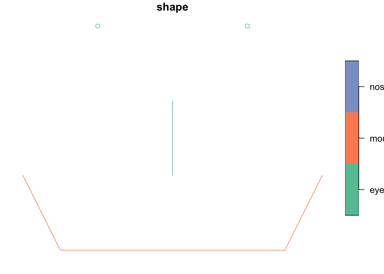

Expand here to see past versions of unnamed-chunk-2-1.png:

Version	Author	Date
0a20853	annakrystalli	2018-09-04

2) What are the coordinates for the 10th point in the Mexico polygon?

mx_coords <- world %>% filter(iso_a2 == "MX") %>% st_coordinates() 

mx_coords[10, c("X", "Y")]

         X          Y 
-106.50759   31.75452

3) How about in CRS Mexico ITRF92 / UTM zone 15N

(hint: use st_transform to change the projection first)

mx_utm15 <- world %>% 
    st_transform(crs = 4488) 

mx_coords <- mx_utm15 %>%
    filter(iso_a2 == "MX") %>% 
    st_coordinates() 

mx_coords[10, c("X", "Y")]

        X         Y 
-784546.6 3593838.9

4) Are these coordinates projected or not? Can you tell by just looking at the CRS in the transformed `sf` object?

mx_utm15

Simple feature collection with 177 features and 10 fields
geometry type:  MULTIPOLYGON
dimension:      XY
bbox:           xmin: -11779910 ymin: -19977280 xmax: 17183260 ymax: 19983850
epsg (SRID):    4488
proj4string:    +proj=utm +zone=15 +ellps=GRS80 +towgs84=0,0,0,0,0,0,0 +units=m +no_defs
First 10 features:
   iso_a2        name_long     continent region_un          subregion
1      FJ             Fiji       Oceania   Oceania          Melanesia
2      TZ         Tanzania        Africa    Africa     Eastern Africa
3      EH   Western Sahara        Africa    Africa    Northern Africa
4      CA           Canada North America  Americas   Northern America
5      US    United States North America  Americas   Northern America
6      KZ       Kazakhstan          Asia      Asia       Central Asia
7      UZ       Uzbekistan          Asia      Asia       Central Asia
8      PG Papua New Guinea       Oceania   Oceania          Melanesia
9      ID        Indonesia          Asia      Asia South-Eastern Asia
10     AR        Argentina South America  Americas      South America
                type    area_km2       pop  lifeExp gdpPercap
1  Sovereign country    19289.97    885806 69.96000  8222.254
2  Sovereign country   932745.79  52234869 64.16300  2402.099
3      Indeterminate    96270.60        NA       NA        NA
4  Sovereign country 10036042.98  35535348 81.95305 43079.143
5            Country  9510743.74 318622525 78.84146 51921.985
6  Sovereign country  2729810.51  17288285 71.62000 23587.338
7  Sovereign country   461410.26  30757700 71.03900  5370.866
8  Sovereign country   464520.07   7755785 65.23000  3709.082
9  Sovereign country  1819251.33 255131116 68.85600 10003.089
10 Sovereign country  2784468.59  42981515 76.25200 18797.548
                             geom
1  MULTIPOLYGON (((-11776327 -...
2  MULTIPOLYGON (((7508185 -19...
3  MULTIPOLYGON (((9294103 882...
4  MULTIPOLYGON (((-1664512 58...
5  MULTIPOLYGON (((-1664512 58...
6  MULTIPOLYGON (((473784.4 14...
7  MULTIPOLYGON (((3108708 149...
8  MULTIPOLYGON (((-6664974 -1...
9  MULTIPOLYGON (((-6664974 -1...
10 MULTIPOLYGON (((2134436 -61...

We’ve already talked about UTM being projected CRSs but there is also a hint in the proj4string, in particular +units=m indicating that the units are linear (m).

We can also extract the units from an sfs crs using function sf::st_crs() and accessing the units

st_crs(mx_utm15)$units

[1] "m"

Raster spatial data

1) Create and plot a new `rasterLayer` of rough mean temperature in degrees C

(rough because it would be much better to use more data at higher temporal resolution, eg at least monthly, not extremes).

We can do this using a simple mean calculation:

rough_mean <- ((full_stack[["mx.bio_5"]] + full_stack[["mx.bio_6"]])/2)/10

But we can even use r functions, in this case mean()

rough_mean <- mean(full_stack[["mx.bio_5"]], full_stack[["mx.bio_6"]])/10

rough_mean

class       : RasterLayer 
dimensions  : 563, 811, 456593  (nrow, ncol, ncell)
resolution  : 0.008333333, 0.008333333  (x, y)
extent      : -101.85, -95.09167, 16.94167, 21.63333  (xmin, xmax, ymin, ymax)
coord. ref. : +proj=longlat +datum=WGS84 +no_defs +ellps=WGS84 +towgs84=0,0,0 
data source : /Users/Anna/Documents/workflows/workshops/intro-r-gis/data/raster/rough_mean.tif 
names       : rough_mean 
values      : -1.45, 29.6  (min, max)

levelplot(rough_mean, margin = F)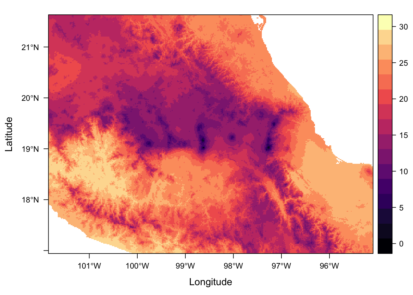

Expand here to see past versions of unnamed-chunk-11-1.png:

Version	Author	Date
0a20853	annakrystalli	2018-09-04

2) Calculate mean precipitation seasonality for the extraction bounding box area. What is the value?

mean_prec_seasonality <- extract(env_stack[["prec_seasonality"]], 
                as_Spatial(extract_bbox),
                fun = mean,
                na.rm = T)

mean_prec_seasonality

         [,1]
[1,] 87.78957

3) Add a column indicating whether data points are greater than (`TRUE`) or less than (`FALSE`) extraction area mean precipitation seasonality.

mol_env_sf <- mol_env_sf %>% 
    mutate(greater_mean_ps = 
               prec_seasonality > as.vector(mean_prec_seasonality))

mol_env_sf %>% select(locality, greater_mean_ps)

Simple feature collection with 15 features and 2 fields
geometry type:  POINT
dimension:      XY
bbox:           xmin: -99.84806 ymin: 18.94194 xmax: -97.09056 ymax: 19.63083
epsg (SRID):    4326
proj4string:    +proj=longlat +datum=WGS84 +no_defs
# A tibble: 15 x 3
   locality               greater_mean_ps             geometry
   <chr>                  <lgl>                    <POINT [°]>
 1 Nevado de Toluca       FALSE           (-99.84806 19.19361)
 2 Texcalyacac            TRUE                (-99.5 19.12056)
 3 Desierto de los Leones TRUE            (-99.30056 19.26667)
 4 Ajusco                 TRUE                (-99.3 19.18278)
 5 Calpan                 TRUE            (-98.59167 19.13139)
 6 Atzompa                TRUE            (-98.55972 19.18056)
 7 Llano Grande           FALSE           (-98.72056 19.33889)
 8 Rio Frio               FALSE           (-98.69472 19.36611)
 9 Nanacamilpa            FALSE           (-98.59611 19.48028)
10 MalincheS              FALSE           (-98.02194 19.18722)
11 MalincheW              FALSE             (-98.095 19.25778)
12 MalincheE              FALSE                (-97.975 19.23)
13 Texmalaquilla          FALSE              (-97.29 18.94194)
14 Xometla                FALSE             (-97.19056 18.975)
15 Vigas                  FALSE           (-97.09056 19.63083)

Session information

sessionInfo()

R version 3.4.4 (2018-03-15)
Platform: x86_64-apple-darwin15.6.0 (64-bit)
Running under: macOS High Sierra 10.13.3

Matrix products: default
BLAS: /Library/Frameworks/R.framework/Versions/3.4/Resources/lib/libRblas.0.dylib
LAPACK: /Library/Frameworks/R.framework/Versions/3.4/Resources/lib/libRlapack.dylib

locale:
[1] en_GB.UTF-8/en_GB.UTF-8/en_GB.UTF-8/C/en_GB.UTF-8/en_GB.UTF-8

attached base packages:
[1] stats     graphics  grDevices utils     datasets  methods   base     

other attached packages:
 [1] bindrcpp_0.2.2      spData_0.2.9.3      ggplot2_3.0.0      
 [4] dplyr_0.7.6         sf_0.6-3            rasterVis_0.45     
 [7] latticeExtra_0.6-28 RColorBrewer_1.1-2  lattice_0.20-35    
[10] raster_2.6-7        sp_1.2-5           

loaded via a namespace (and not attached):
 [1] zoo_1.8-3         tidyselect_0.2.4  purrr_0.2.5      
 [4] colorspace_1.3-2  htmltools_0.3.6   viridisLite_0.3.0
 [7] yaml_2.1.19       utf8_1.1.3        rlang_0.2.1      
[10] R.oo_1.21.0       e1071_1.6-8       hexbin_1.27.1    
[13] pillar_1.2.1      glue_1.2.0.9000   withr_2.1.2      
[16] DBI_1.0.0         R.utils_2.6.0     bindr_0.1.1      
[19] plyr_1.8.4        stringr_1.3.1     munsell_0.5.0    
[22] gtable_0.2.0      workflowr_1.0.1   R.methodsS3_1.7.1
[25] evaluate_0.11     knitr_1.20        parallel_3.4.4   
[28] class_7.3-14      Rcpp_0.12.18      backports_1.1.2  
[31] scales_1.0.0      classInt_0.1-24   digest_0.6.15    
[34] stringi_1.2.4     grid_3.4.4        rprojroot_1.3-2  
[37] cli_1.0.0         rgdal_1.3-4       here_0.1         
[40] tools_3.4.4       magrittr_1.5      lazyeval_0.2.1   
[43] tibble_1.4.2      crayon_1.3.4      whisker_0.3-2    
[46] pkgconfig_2.0.2   assertthat_0.2.0  rmarkdown_1.10   
[49] R6_2.2.2          units_0.6-0       git2r_0.21.0     
[52] compiler_3.4.4

This reproducible R Markdown analysis was created with workflowr 1.0.1