1 The Fitch algorithm
This algorithm was proposed by Fitch (1971) and is implemented in many phylogenetic softwares based on maximum parsimony (Goloboff & Catalano, 2016; Swofford, 2001) or probabilistic methods (Ronquist et al., 2012; Stamatakis, 2014). The procedure is simple and elegant and entails going down the tree to count the number of transformations, and then going back up the tree to finalise the ancestral state reconstructions.
The way the algorithm goes up and down depends on the software, but often employs a traversal: a recursive function that can visit all tips and nodes in a logical fashion. For example, consider the following tree:
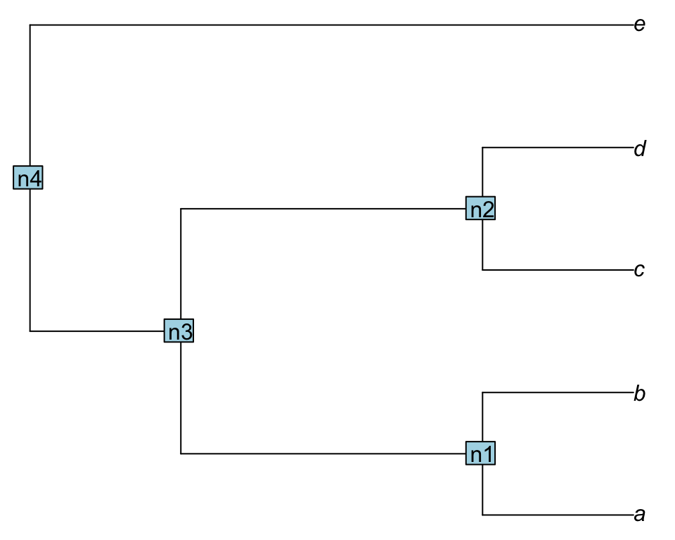
Figure 1.1: A five-tip tree
A downpass traversal will first evaluate the first cherry (or pair of taxa) (A below), then save the results in n1 and evaluate the second pair of tips/nodes (B), saving the results in n2, proceeding until all the nodes/tips are visited.
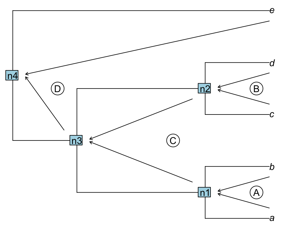
Figure 1.2: Downpass traversal
An uppass traversal works identically but in the other direction, going from the nodes towards the tips.
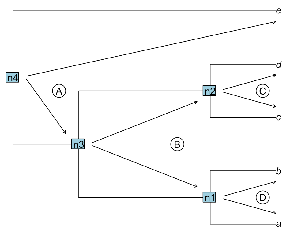
Figure 1.3: Uppass traversal
In both traversals, the sequence in which nodes are visited (i.e. which cherry to pick first in a downpass traversal, or whether to continue left or right in an uppass traversal) is arbitrary, provided that all tips and nodes are eventually visited.
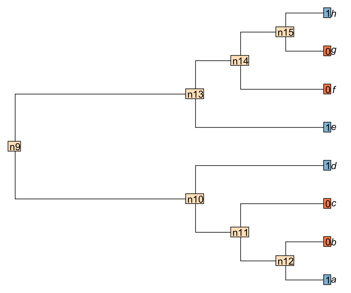
Now let’s consider a more complex tree ((((a, b), c), d), (e, (f, (g, h)))); with a binary character distributed ((((1, 0), 0), 1), (1, (0, (0, 1)))):
We can use the Inapp package to apply the Fitch algorithm for this character on this tree.
## Loading the Inapp package
library(Inapp)

## The tree
tree <- read.tree(text = "((((a, b), c), d), (e, (f, (g, h))));")

## The character
character <- "10011001"

## Applying the Fitch algorithm
matrix <- apply.reconstruction(tree, character, method = "Fitch", passes = 2)
1.1 Downpass
The downpass is quite simple and follows these rules for the two possible cases in the traversal:
- If the two considered tips or nodes have at least one state in common, set the node to be these states in common.
- Else, if there is nothing in common between the to tips or nodes, set the node to be the union of the two states.
For example, node n15 is case 2 because there is nothing in common between the tips h and g (states 1 and 0 respectively). Node n14 is case 1 because there is at least one state in common between the tip f and the node n15 (state 0).
Important: when the case 2 is encountered, a transformation is implied in the descendants of the considered node. The score of the tree is incremented by +1.
In the following example, nodes that are in case 1 are in white and nodes in case 2, which imply a transformation (i.e. that adds to the tree score), are in green.
## Plotting the first downpass
plot.states.matrix(matrix, passes = 1, counts = 2, show.labels = c(1,2))
tiplabels(char, cex = 1, bg = Inapp::brewer[[2]][char + 1], adj = 1)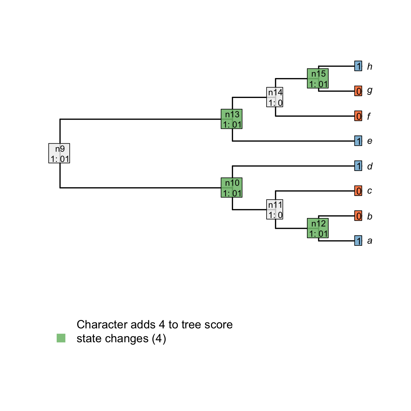
Figure 1.4: Node reconstructions after downpass
1.2 Uppass
The score of the tree is known after the downpass, but the states of some nodes might not yet be properly resolved. For example, parsimonious reconstructions exist that reconstruct node n14 as state 1, as opposed to the 0 presently reconstructed. The present reconstruction seemingly indicates a change from state 1 to state 0 in an ancestor of n14, and a subsequent change from state 0 to state 1 in the ancestor of h, but an alternative reconstruction is equally parsimonious: n13, n14 and n15 may all have state 1, with a change from state 1 to state 0 in each of the two lineages leading to f and g.
The uppass traversal employs the following rules:
- If the current node and its ancestor have all states in common, the node is already resolved.
- If there is at least one state in common between both left and right tips or nodes directly descended from the current node, resolve the node as being the states in common between its ancestor and both his descendants.
- If there is there are no states in common between its descendants, resolve the node as being the states in common between the ancestor and the current node.
For example, node n13 is already resolved (it has all its states in common with the ancestor - case 1). Node n14 has not all its states in common with its ancestor but its two descendants (n15 and f) have at least one state in common (0). This node is thus solved to be the states in common between both descendants (01) and its ancestor (01 as well).
## Plotting the first uppass
plot.states.matrix(matrix, passes = 1:2, counts = 2,
                   show.labels = c(1, 2), col.states=TRUE)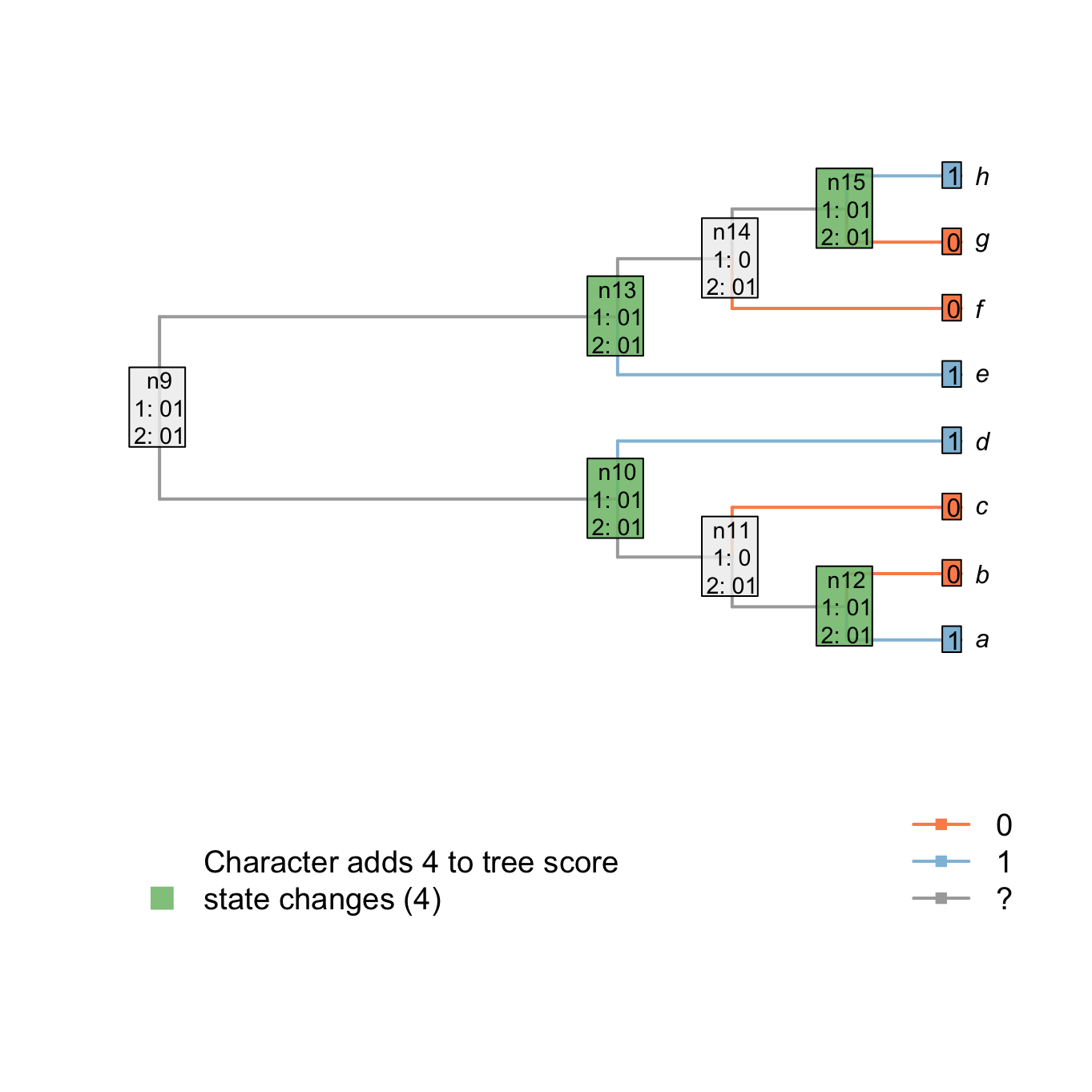
Figure 1.5: Node reconstructions after uppass
More complex cases can be studied in the Inapp App (running in your favourite web browser) by switching the Reconstruction method to Normal Fitch.
## Running the Inapp App
runInapp()
1.3 Resolving ambiguous resolutions
In certain cases, it is necessary to go further and discriminate between the equally-parsimonious reconstructions provided by the Fitch algorithm. A number of approaches have been proposed concerning which resolution of ambiguous nodes is preferable.
The two most familiar approaches to resolving ambiguous node are the Accelerated Transformation (AccTran) and Delayed Transformation (DelTran) approaches.
The AccTran approach reconstructs transformations as occurring as close to the root as possible; the DelTran, as far from the root as possible.
In this case, the ambiguous resolution of the root leaves two options for the latter:
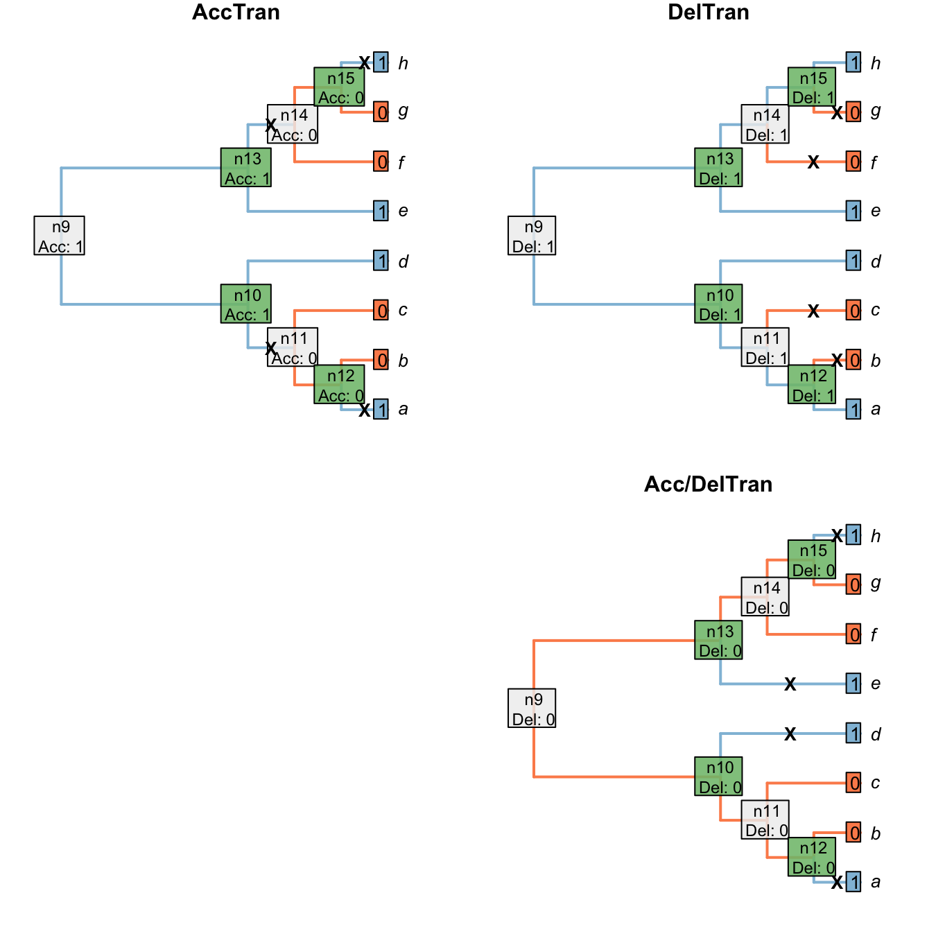
Figure 1.6: Node reconstructions after AccTran or DelTran` optimizations
If the states 0 and 1 represent states of a transformational character – whether an organism’s tail is red or blue, say – then there is no reason to prefer any of the equally-parsimonious reconstructions, as none implies any more homology than any other.
With neomorphic characters, however, state 0 stands for the absence of a character – for example, a tail – and state 1 its presence. On one view, a reconstruction that minimises the number of times that such a character evolves attributes more similarity to homology than an equally parsimonious reconstruction in which said character is gained multiple times independently.
1.3.1 Maximising homology
Neither AccTran nor DelTran is guaranteed to maximise homology (Agnarsson & Miller, 2008). In this particular case, the DelTran reconstruction maximises homology. If the character denotes the presence or absence of a tail, then this reconstruction invokes the presence of a tail in the common ancestor of all taxa, meaning that the tails present in tips a, d, e and h are homologous with one another. The AccTran reconstruction, in contrast, identifies a loss of a tail at nodes 11 and 14, with a tail evolving independently in tips a and h. Under this reconstruction, the tails of a and h are not homologous with each other, or with the tails of d and e. (The alternative DelTran approach, which could arguably be described as AccTran instead, invokes four independent origins of the character and clearly does not maximise its homology.)
Where we wish to maximise homology, we modify the Fitch uppass such that any node whose final state reconstruction would be ambiguous is instead reconstructed as present when that node is encountered. This approach maximises homology in the problematic trees presented by Agnarsson & Miller (2008)(“A&M” below):
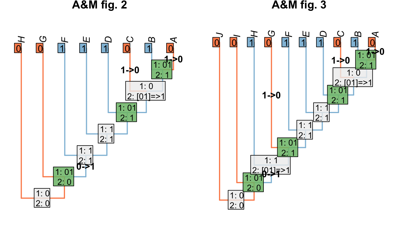
Figure 1.7: Homology-maximising character optimisations
This approach is also robust to missing entries:
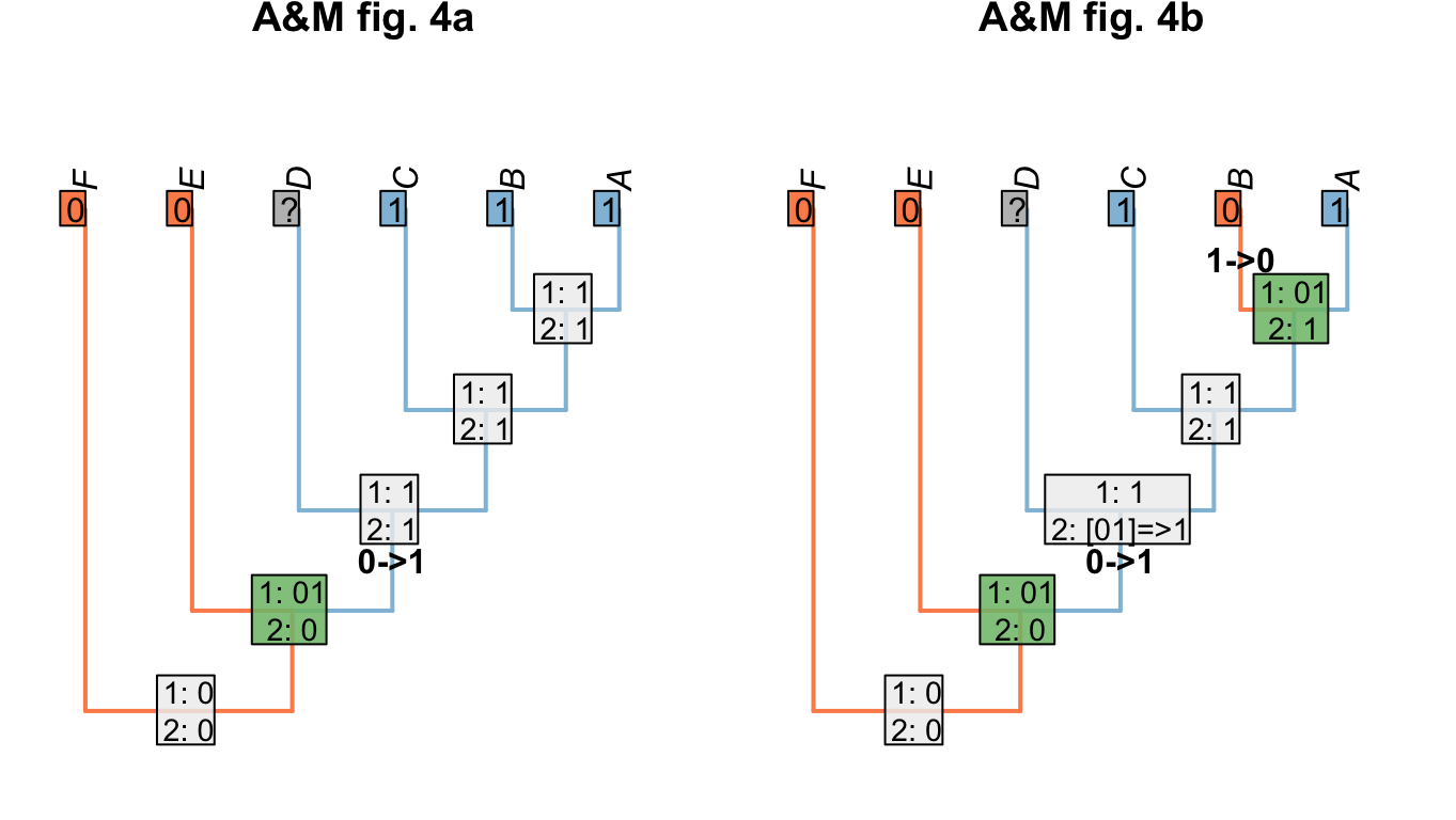
Figure 1.8: Homology maximisation with missing entries
References
Fitch, W. M. (1971). Toward defining the course of evolution: minimum change for a specific tree topology. Systematic Biology, 20(4), 406–416. doi:10.1093/sysbio/20.4.406
Goloboff, P. A., & Catalano, S. A. (2016). TNT version 1.5, including a full implementation of phylogenetic morphometrics. Cladistics, 32(3), 221–238. doi:10.1111/cla.12160
Swofford, D. L. (2001). PAUP*: Phylogenetic analysis using parsimony (and other methods) 4.0. B5.
Ronquist, F., Teslenko, M., Mark, P. van der, Ayres, D. L., Darling, A., Hohna, S., … Huelsenbeck, J. P. (2012). MrBayes 3.2: Efficient Bayesian phylogenetic inference and model choice across a large model space. Systematic Biology, 61(3), 539–42.
Stamatakis, A. (2014). RAxML version 8: A tool for phylogenetic analysis and post-analysis of large phylogenies. Bioinformatics, 30(9), 1312–1313. doi:10.1093/bioinformatics/btu033
Agnarsson, I., & Miller, J. A. (2008). Is AccTran better than DelTran? Cladistics, 24(6), 1032–1038. doi:10.1111/j.1096-0031.2008.00229.x