6 Examples
This vignette describes how the algorithm approaches some example trees. We follow the example of a tail coded using two characters:
Tail: (0), absent; (1), present;
Tail colour: (0), red; (1), blue.
6.1 Some caterpillars
First we’ll address some pectinate “caterpillar” trees, in which eight taxa have tails (and eight do not), four of which are red, four of which are blue.
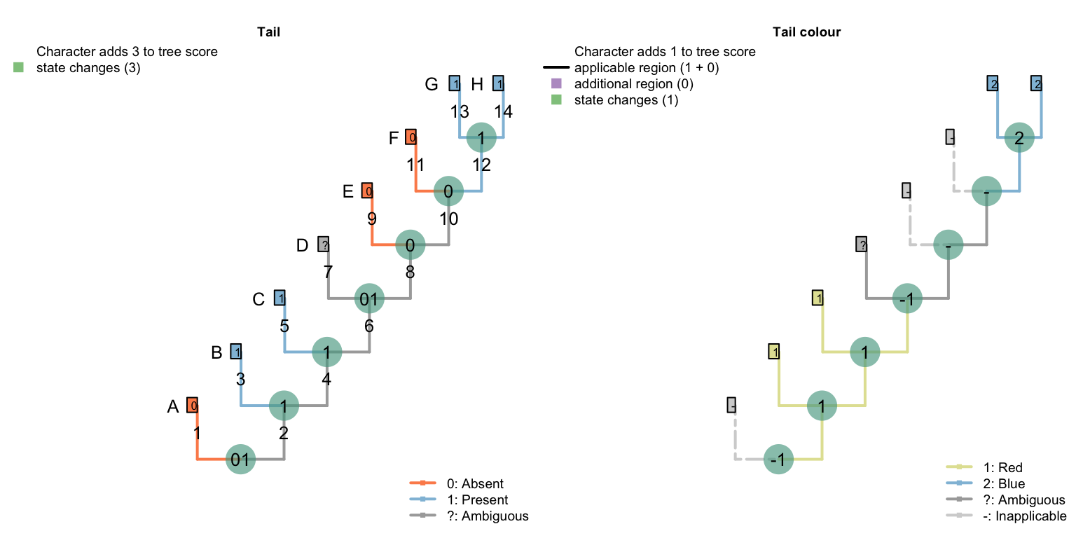
An optimal tree with this character invokes a single origin of the tail, and a single change in tail colour, thus incurring a score of two. Here is one example:
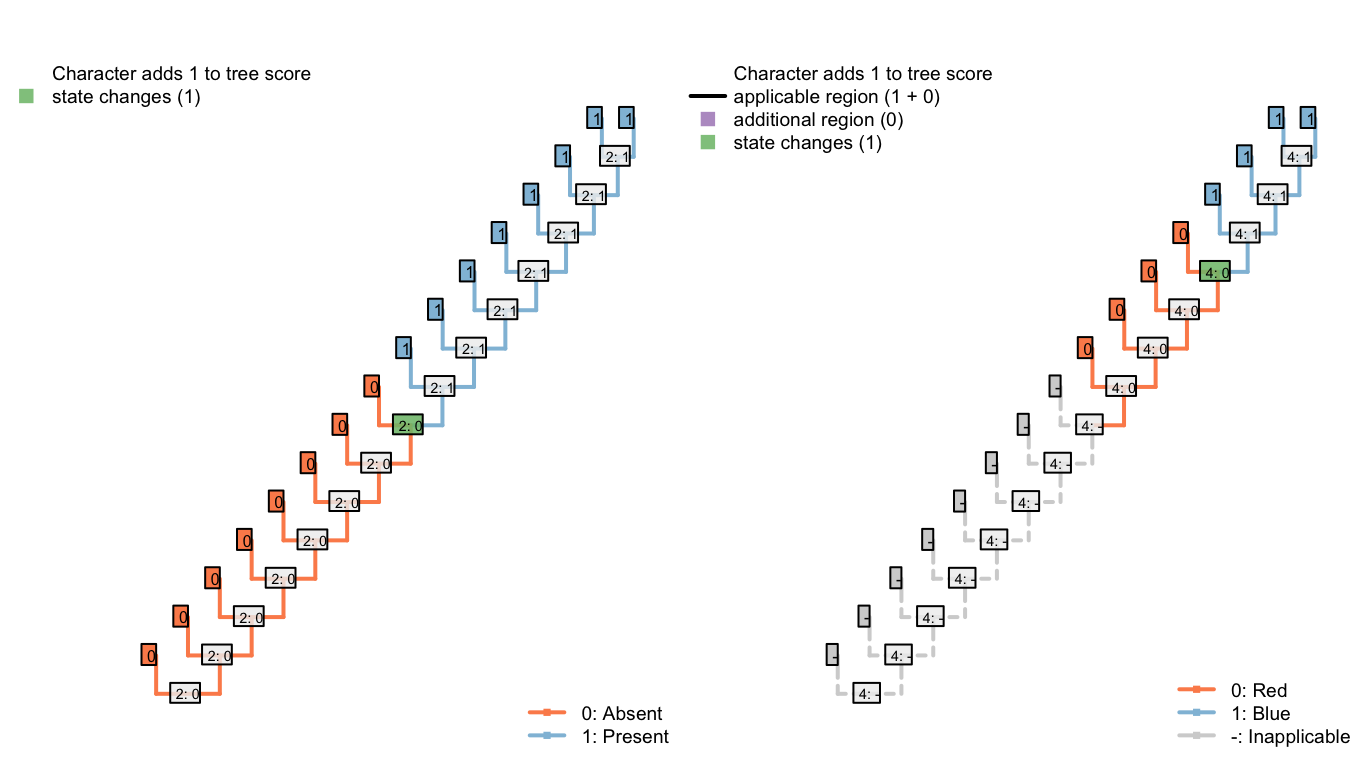
Figure 6.1: An optimal tree: Total score 2
If we insist that the tail evolves twice, then the best score is accomplished by reconstructing a different colour of tail in each of the two regions in which the tail is present. On a caterpillar tree, this means the loss of a tail that has one colour, and an independent innovation in a tail-less taxon of a tail that has a different colour:
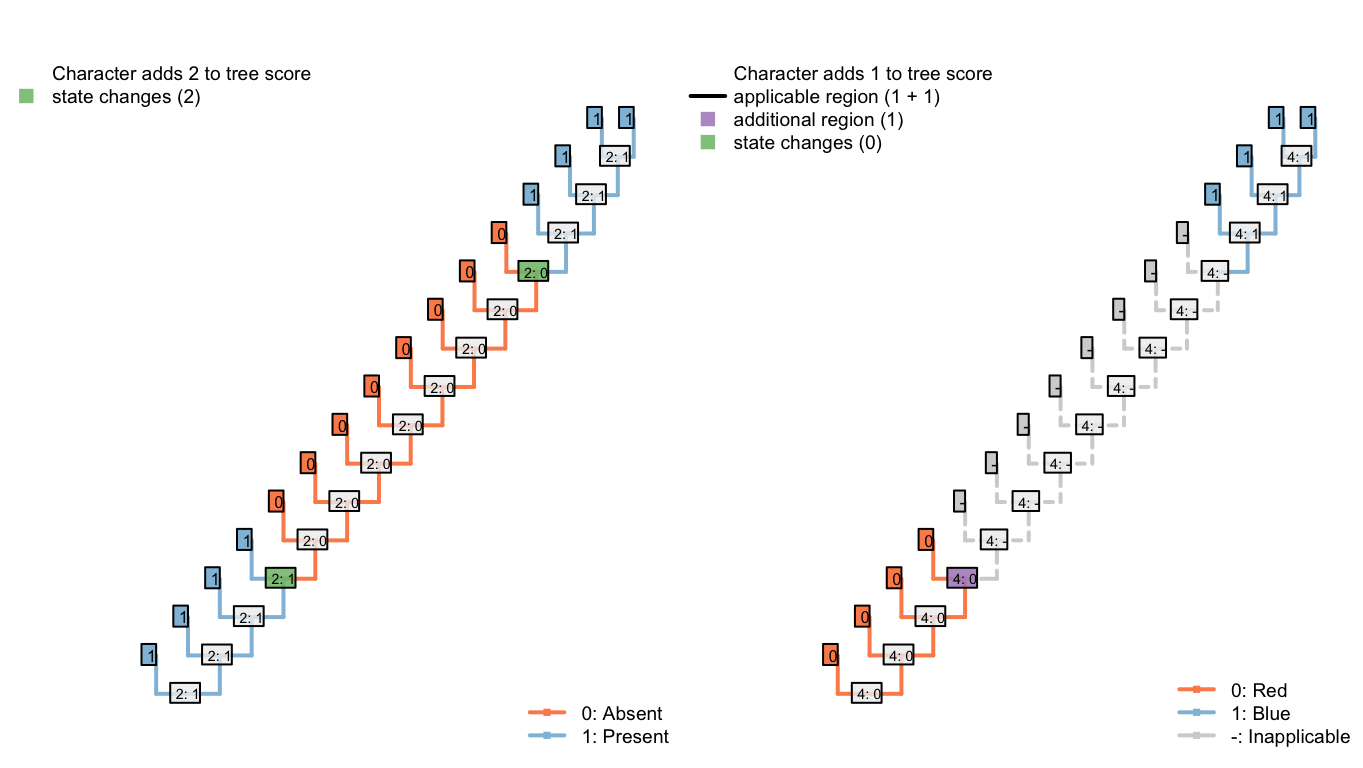
Figure 6.2: Two tail innovations: Total score 2 (best possible)
Under the parsimony criterion, it is considered less optimal if a tail, when it re-evolves, happens to independently re-evolve a colour that has already been observed – “blueness” has evolved twice on the following tree, meaning that the second innovation of “blueness” represents an instance of homoplasy.
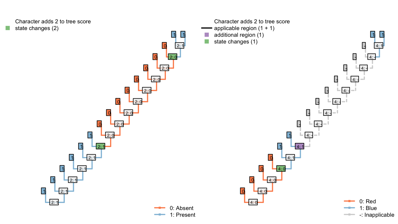
Figure 6.3: Tree A: Total score 4
6.2 Three equally suboptimal alternatives
The following three trees differ in the number of innovations of the tail that are implied, and the number of changes in tail colour. All are equally parsimonious.
Under the first, our algorithm reconstructs the tail as ancestrally present, being lost on edge 2, gained on edge 5, lost in tips H and I, lost on edge 11, and gained on edge 14 (a total of six homoplasies). It further reconstructs independent, homoplastic origins of tail redness on edge 5, tail blueness on edge 14, and a change in tail colour from red to blue somewhere between edges 7 and 9 (three homoplasies).
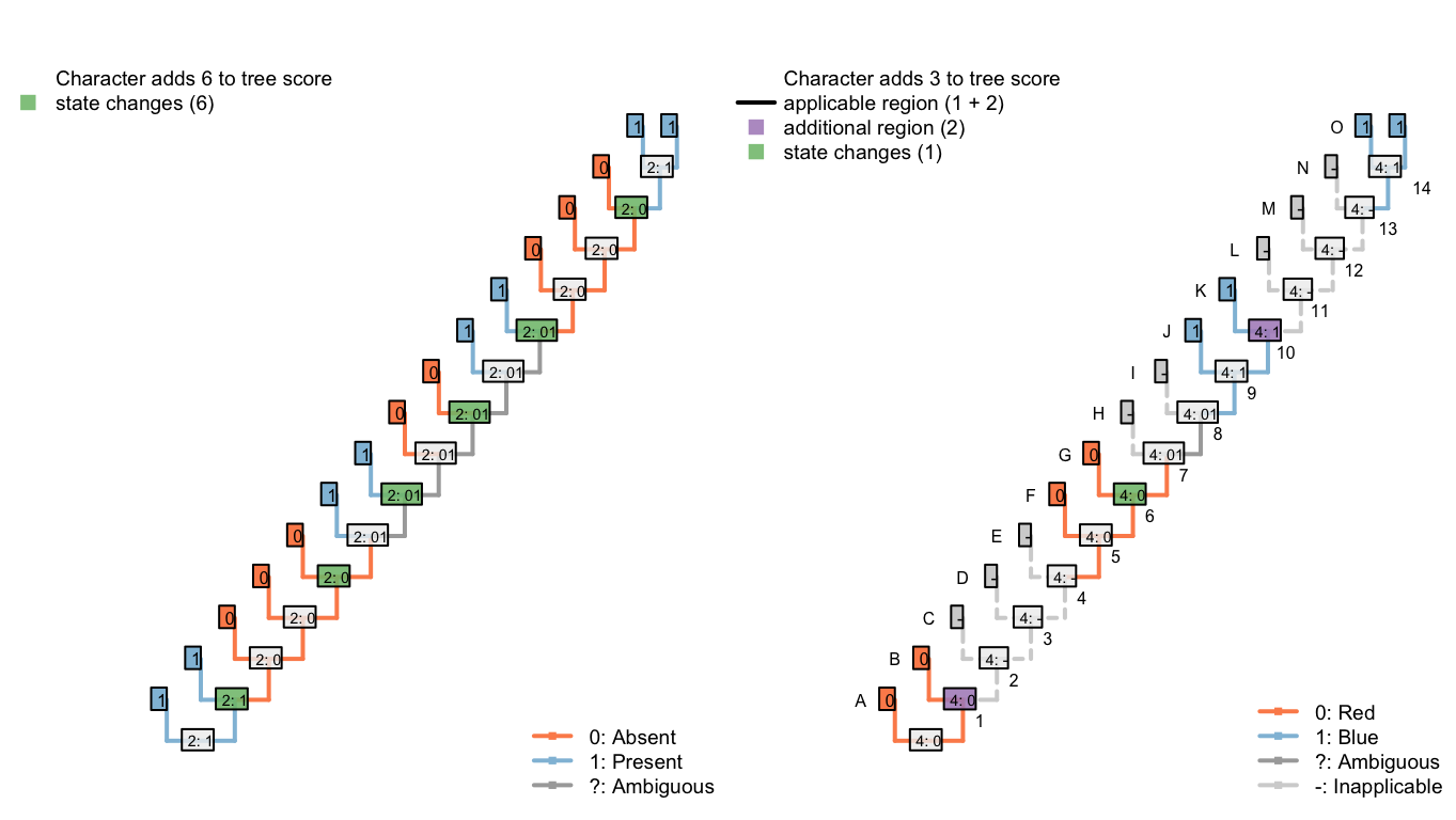
Figure 6.4: Tree B: Total score 9
In the second, our algorithm reconstructs the tail as ancestrally present, being lost in tips B, D, E, H, and I, and on edge 11, before being independently gained on edge 14 (a total of seven homoplasies).
It further reconstructs an independent, homoplastic origins of tail blueness on edge 14, and a change in tail colour from red to blue somewhere between edges 7 and 9 (two homoplasies).
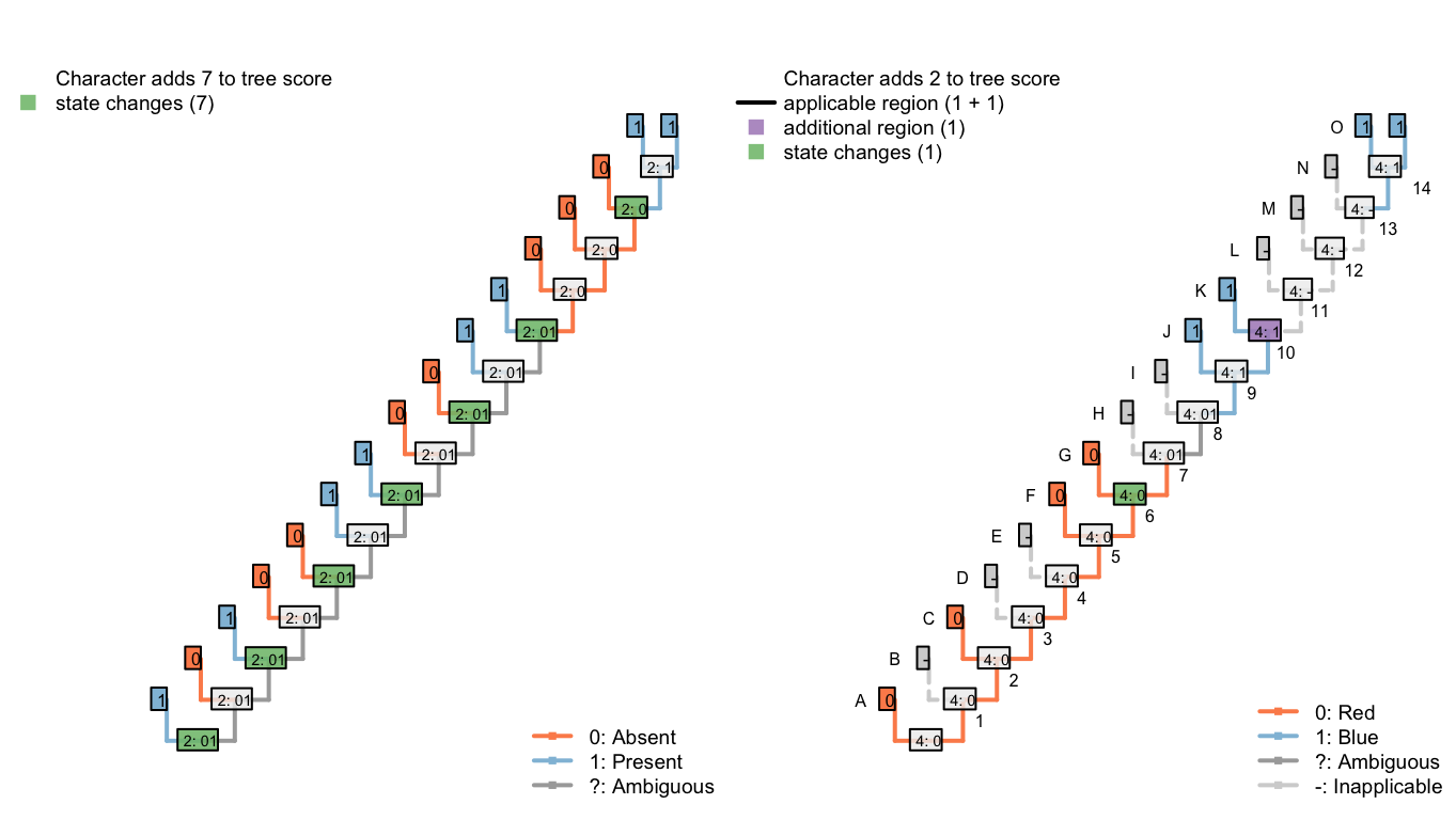
Figure 6.5: Tree C: Total score 9
The third configuration reconstructs the tail as ancestrally present, being lost in tips B, D, F, H, J, L, N and P (a total of eight homoplastic losses). It further reconstructs a single change in tail colour from red to blue on edge 8.
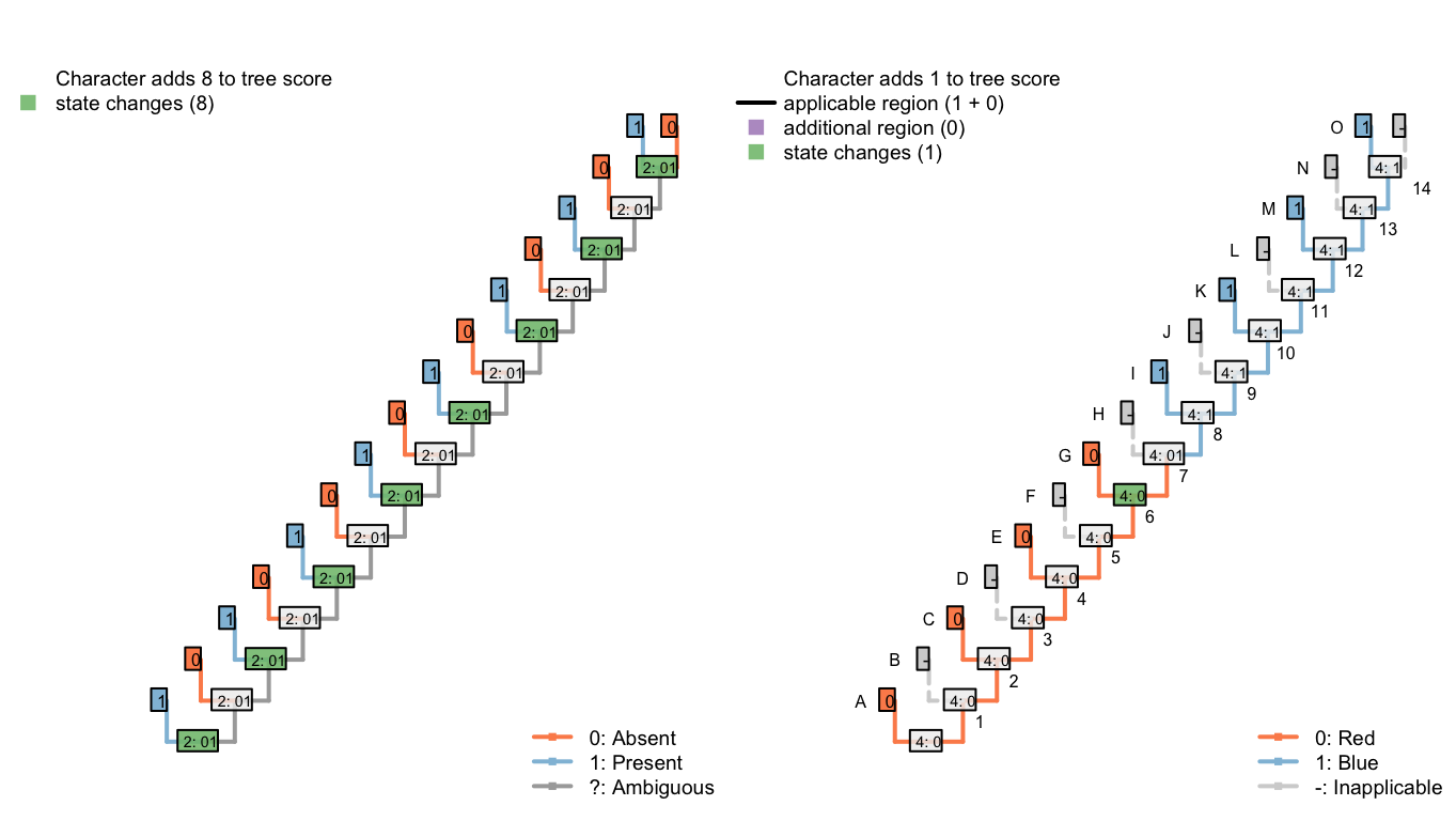
Figure 6.6: Tree D: Total score 9
6.3 A better caterpillar tree
The tree below obtains a better score than any of the previous three: it implies a loss of the tail at edge 2, a gain at edge 6, a loss at edge 10, and a gain at edge 14; it invokes a homoplastic origin of redness at edge 6, one of blueness at edge 14, and a change in colour at edge 8, for a combined score of 7.
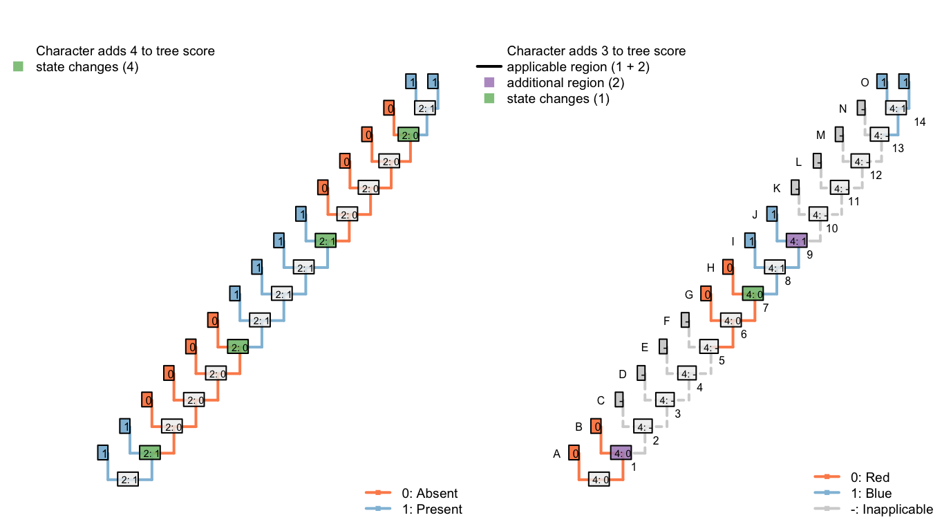
Figure 6.7: Tree E: Total score 7
6.4 De Laet’s caterpillars
De Laet (2017) identifies a corner case in which our algorithm (Brazeau et al., 2017) will not reconstruct every equally-parsimonious character reconstruction. Below is a simplified version of his example:
| A | B | C | D | E | F | G | H | |
|---|---|---|---|---|---|---|---|---|
| Tail: (0), absent; (1), present. | 0 | 1 | 1 | ? | 0 | 0 | 1 | 1 |
| Tail, colour: (1), red; (2),blue. | - | 1 | 1 | ? | - | - | 2 | 2 |
When optimising tail colour, we reconstruct the tail as present at all internal nodes, with independent losses of the tail in each of the three tailless taxa (i.e. edges 1, 9, 11).

The Fitch algorithm identifies other reconstructions as equally parsimonious: for example, a tail may have been lost on edge 6 and re-gained on edge 12. This also incurs three steps for the tail character, and (in De Laet’s parlance) attributes three similarities to common ancestry: the presence of a tail in tips B and C, the absence of the tail in tips E and F, and the presence of a tail in tips G and H.
We prefer reconstructions that attribute the presence of a feature to common ancestry where possible – a philosophy that shares something with Dollo’s contention that it is easier to lose a feature than to gain it. On a pragmatic level, this maximises the opportunity for subsidiary traits of the tail to be attributed to common ancestry.
In this particular case, there is an equally-parsimonious character reconstruction that our algorithm excludes, which invokes two gains (and one loss) of the tail:
This has no effect on tree scoring, but may be relevant if complete internal nodal reconstructions are desired.
References
De Laet, J. (2017). A note on Brazeau et al.’s (2017) algorithm for characters with inapplicable data, illustrated with an analysis of their Fig. 3d using anagallis, a program for parsimony analysis of character hierarchies. doi:10.13140/RG.2.2.31309.54245
Brazeau, M. D., Guillerme, T., & Smith, M. R. (2017). Morphological phylogenetic analysis with inapplicable data. bioR\(\chi\)iv. doi:10.1101/209775