Drop-seq Example
Last updated: 2018-08-29
workflowr checks: (Click a bullet for more information)-
✔ R Markdown file: up-to-date
Great! Since the R Markdown file has been committed to the Git repository, you know the exact version of the code that produced these results.
-
✔ Environment: empty
Great job! The global environment was empty. Objects defined in the global environment can affect the analysis in your R Markdown file in unknown ways. For reproduciblity it’s best to always run the code in an empty environment.
-
✔ Seed:
set.seed(20180618)The command
set.seed(20180618)was run prior to running the code in the R Markdown file. Setting a seed ensures that any results that rely on randomness, e.g. subsampling or permutations, are reproducible. -
✔ Session information: recorded
Great job! Recording the operating system, R version, and package versions is critical for reproducibility.
-
Great! You are using Git for version control. Tracking code development and connecting the code version to the results is critical for reproducibility. The version displayed above was the version of the Git repository at the time these results were generated.✔ Repository version: 9203702
Note that you need to be careful to ensure that all relevant files for the analysis have been committed to Git prior to generating the results (you can usewflow_publishorwflow_git_commit). workflowr only checks the R Markdown file, but you know if there are other scripts or data files that it depends on. Below is the status of the Git repository when the results were generated:
Note that any generated files, e.g. HTML, png, CSS, etc., are not included in this status report because it is ok for generated content to have uncommitted changes.Ignored files: Ignored: .Rhistory Ignored: .Rproj.user/ Ignored: R/.Rhistory Ignored: analysis/.Rhistory Ignored: analysis/pipeline/.Rhistory Untracked files: Untracked: ..gif Untracked: .DS_Store Untracked: R/.DS_Store Untracked: R/myheatmap.R Untracked: analysis/.DS_Store Untracked: analysis/Dropseqpreprocessing_cache/ Untracked: analysis/SLSL_marker_based_logcpm.pdf Untracked: analysis/biomarkers.R Untracked: analysis/cellref.pdf Untracked: analysis/consistency_check.R Untracked: analysis/dropseq_sc3_result.Rdata Untracked: analysis/dropseq_slsl1.Rdata Untracked: analysis/example_smartseq.Rmd Untracked: analysis/marker-based.pdf Untracked: analysis/normalization_test.R Untracked: analysis/pbmcheat.pdf Untracked: analysis/pbmcref.pdf Untracked: analysis/pipeline/0_dropseq/ Untracked: analysis/pipeline/1_10X/ Untracked: analysis/pipeline/2_zeisel/ Untracked: analysis/pipeline/3_smallsets/ Untracked: analysis/writeup/cite.log Untracked: analysis/writeup/paper.aux Untracked: analysis/writeup/paper.bbl Untracked: analysis/writeup/paper.blg Untracked: analysis/writeup/paper.log Untracked: analysis/writeup/paper.out Untracked: analysis/writeup/paper.synctex.gz Untracked: analysis/writeup/paper.tex Untracked: analysis/writeup/writeup.aux Untracked: analysis/writeup/writeup.bbl Untracked: analysis/writeup/writeup.blg Untracked: analysis/writeup/writeup.dvi Untracked: analysis/writeup/writeup.log Untracked: analysis/writeup/writeup.out Untracked: analysis/writeup/writeup.synctex.gz Untracked: analysis/writeup/writeup.tex Untracked: analysis/writeup/writeup2.aux Untracked: analysis/writeup/writeup2.bbl Untracked: analysis/writeup/writeup2.blg Untracked: analysis/writeup/writeup2.log Untracked: analysis/writeup/writeup2.out Untracked: analysis/writeup/writeup2.pdf Untracked: analysis/writeup/writeup2.synctex.gz Untracked: analysis/writeup/writeup2.tex Untracked: analysis/writeup/writeup3.aux Untracked: analysis/writeup/writeup3.log Untracked: analysis/writeup/writeup3.out Untracked: analysis/writeup/writeup3.synctex.gz Untracked: analysis/writeup/writeup3.tex Untracked: data/unnecessary_in_building/ Untracked: docs/figure/example_10x.Rmd/ Untracked: normalized_out_1.Rdata Untracked: not_normalized_out_1.Rdata Untracked: src/.gitignore Untracked: tutorial2.Rmd Unstaged changes: Modified: NAMESPACE Modified: R/RcppExports.R Deleted: analysis/10Xpreprocessing.Rmd Deleted: analysis/Dropseqpreprocessing.Rmd Modified: analysis/about.Rmd Modified: analysis/license.Rmd Modified: analysis/pipeline/.DS_Store Modified: analysis/writeup/.DS_Store Modified: data/.DS_Store
Read data.
library(data.table)
tmp = setDF(fread('data/unnecessary_in_building/GSM1626794_P14Retina_2.digital_expression.txt'))
orig = tmp[,-1]; rownames(orig) = tmp[,1]; rm(tmp)
genenames = sapply(strsplit(rownames(orig), ":"), function(x) x[3])
gc(verbose=FALSE);
used (Mb) gc trigger (Mb) limit (Mb) max used (Mb)
Ncells 2789945 149 4252298 227.1 NA 4252298 227.1
Vcells 106685452 814 155388100 1185.6 16384 107643487 821.3Quality Control and Cell Filter
nGene = colSums(orig > 0)
hist(nGene)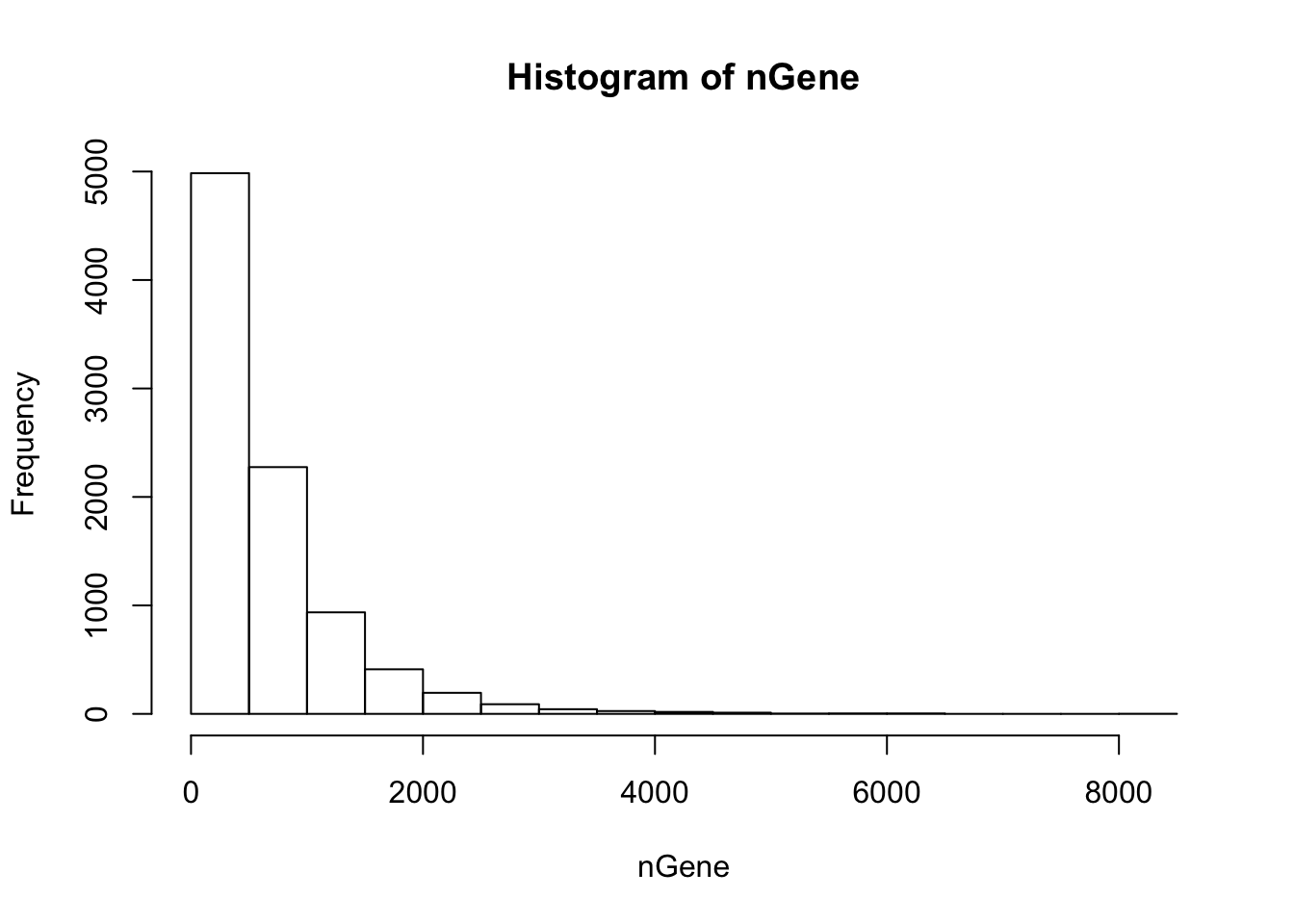
summaryX = cellFilter(X = orig,
                      genenames = genenames,
                      minGene = 500,
                      maxGene = 2000,
                      maxMitoProp = 0.1)
tmpX = summaryX$X
nUMI = summaryX$nUMI
nGene = summaryX$nGene
percent.mito = summaryX$percent.mito
det.rate = summaryX$det.rate

par(mfrow = c(1,4))
boxplot(nUMI, main='nUMI');
boxplot(nGene, main='nGene');
boxplot(percent.mito, main='mitochondrial gene', ylim=c(0,0.5));
boxplot(det.rate, main='detection rate', ylim=c(0,0.1))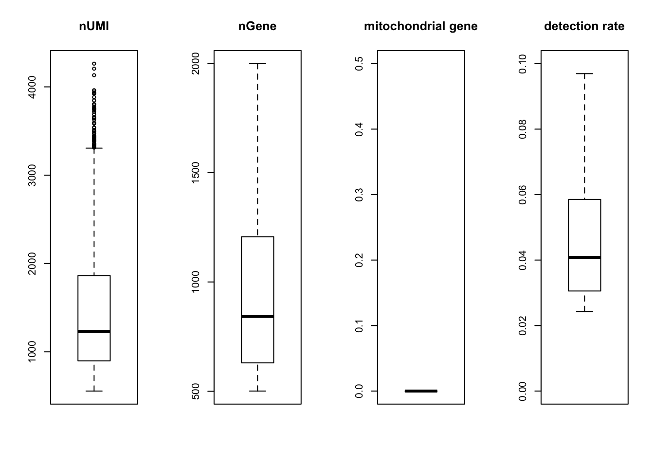
Gene filtering
X = tmpX[rowSums(tmpX) > 0, ]
genenames = genenames[rowSums(tmpX) > 0]

#gene filter by dispersion
disp = dispersion(X, bins = 20)
plot(disp$z ~ disp$genemeans,
     xlab = "mean expression",
     ylab = "normalized dispersion")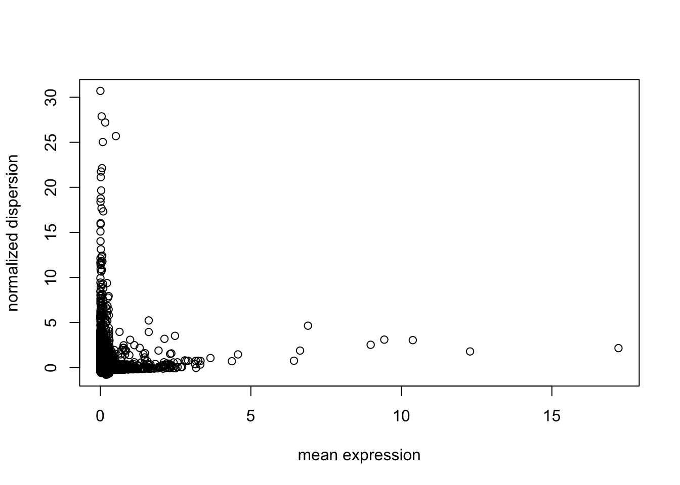
select = which(abs(disp$z) > 1)
X = X[select, ]
genenames = genenames[select]
UMI Normalization
Use quantile-normalization to make the distribution of each cell the same.
nX = quantile_normalize(as.matrix(X))Correct Detection Rate
After normalization, the linear relationship between the first PC and the detection rate usually disappears. The plots show that even without correction, the two are not heavily correlated. So we do not regress out the detection rate.
#take log
logX = as.matrix(log(nX + 1))

#check dependency
out = correct_detection_rate(logX, det.rate)![]()
#regress out
# log.cpm = out$residual
log.cpm = logX
Dimension reduction on the data for visualization.
pc = irlba(log.cpm, 20)
plot(pc$d, ylab = "singular values")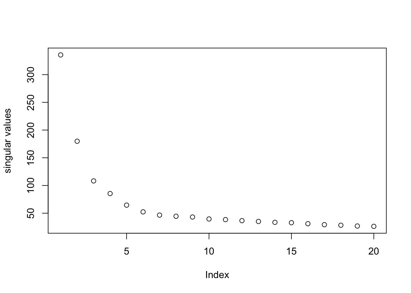
tsne = Rtsne(pc$v[,1:5], dims=2, perplexity = 100, pca=FALSE)
plot(tsne$Y, xlab = 'tsne1', ylab = 'tsne2', cex = 0.5)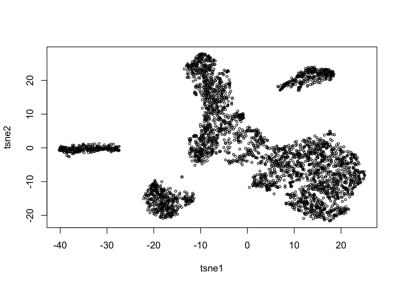
rm(pc)Run SLSL on the log.cpm matrix.
# out = SLSL(log.cpm, log=FALSE,
#                 filter = FALSE,
#                 correct_detection_rate = FALSE,
#                 klist = c(300,350,400),
#                 sigmalist = c(1,1.5,2),
#                 kernel_type = "pearson",
#                 verbose=FALSE)
# save(out, file = 'dropseq_slsl1.Rdata')
load('analysis/dropseq_slsl1.Rdata')
tab = table(out$result)
plot(tsne$Y, col=rainbow(length(tab))[out$result],
     xlab = 'tsne1', ylab='tsne2', main="SLSL", cex = 0.5)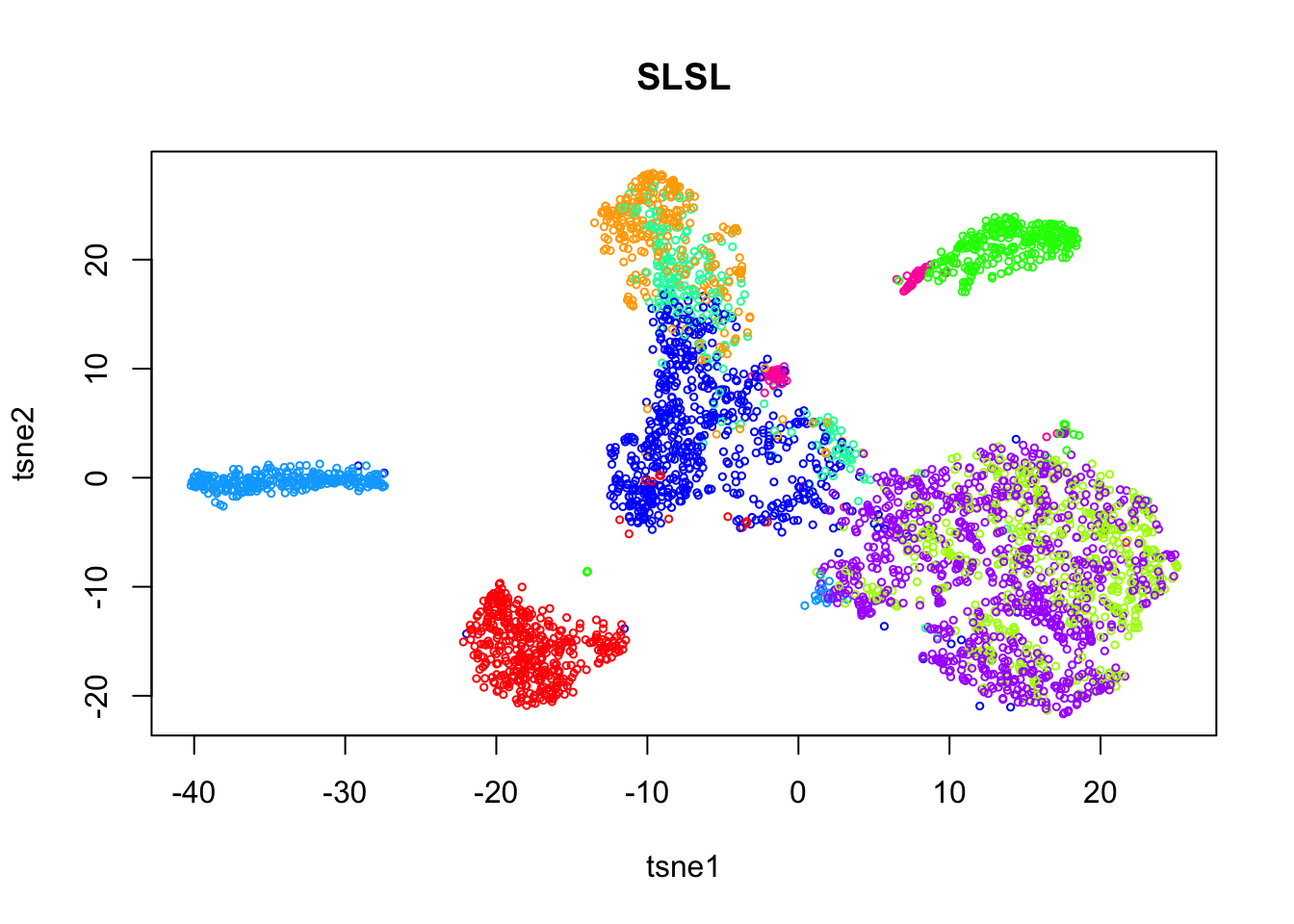
Using SC3 with our gene and cell filter procedure and disabling the biology and filter feature of the function leads to the following result. Using SC3’s default methods lead to the error “distribution of gene expression in cells is too skewed towards 0”.
library(SingleCellExperiment)
library(SC3)
# colnames(X) = paste0("C", 1:ncol(X))
# sce = SingleCellExperiment(
#   assays = list(
#     counts = X,
#     logcounts = as.matrix(log(X+1))
#   ),
#   colData = colnames(X)
# )
# rowData(sce)$feature_symbol = genenames
# sce = sc3_prepare(sce, kmeans_nstart = 50)
# sce = sc3_estimate_k(sce)
# k = metadata(sce)$sc3$k_estimation
# N = ncol(X)
# sce = sc3(sce, ks=k, biology = FALSE, gene_filter=FALSE,
#          kmeans_nstart=10)
# col_data_selected = colData(sce)
# save(col_data_selected, file  = "analysis/dropseq_sc3_result.Rdata")
load('analysis/dropseq_sc3_result.Rdata')
plot(tsne$Y, col=rainbow(k)[col_data_selected$sc3_6_clusters],
     xlab = 'tsne1', ylab='tsne2', main="SC3", cex = 0.5)
ind = which(genenames %in% c('Chat', 'Gad1', 'Gad2', 'Slc17a8', 'Slc6a9', 'Gjd2'))
df = data.frame(tsne1 = tsne$Y[,1], tsne2 = tsne$Y[,2],
Slc17a8 = log.cpm[ind[1], ],
Gad2 = log.cpm[ind[2], ],
Gad1 = log.cpm[ind[3],]
)
g1 = ggplot(df, aes(x=tsne1, y=tsne2, col = Slc17a8)) + geom_point(size=0.1) +
scale_colour_gradient(low="pink", high="black") + guides(color = FALSE) + ggtitle('Slc17a8')
g2 = ggplot(df, aes(x=tsne1, y=tsne2, col = Gad2)) + geom_point(size=0.1) +
scale_colour_gradient(low="pink", high="black") + guides(color = FALSE) + ggtitle('Gad2')
g3 = ggplot(df, aes(x=tsne1, y=tsne2, col = Gad1)) + geom_point(size=0.1) +
scale_colour_gradient(low="pink", high="black") + guides(color = FALSE) + ggtitle('Gad1')
grid.arrange(g1,g2,g3, nrow=1)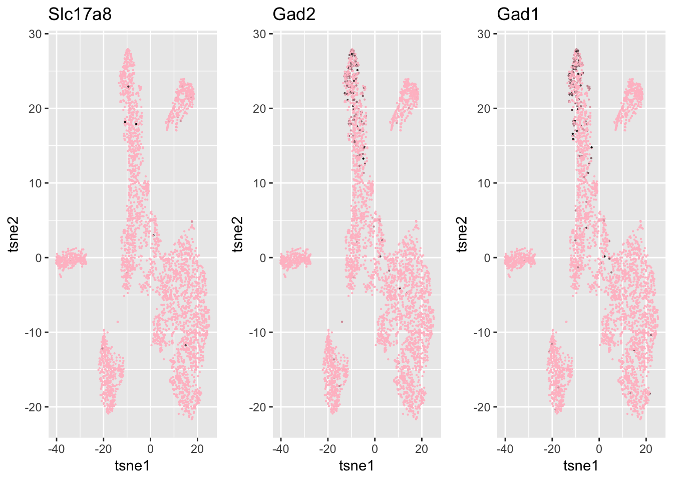
Session information
sessionInfo()R version 3.5.1 (2018-07-02)
Platform: x86_64-apple-darwin15.6.0 (64-bit)
Running under: macOS Sierra 10.12.5
Matrix products: default
BLAS: /Library/Frameworks/R.framework/Versions/3.5/Resources/lib/libRblas.0.dylib
LAPACK: /Library/Frameworks/R.framework/Versions/3.5/Resources/lib/libRlapack.dylib
locale:
[1] en_US.UTF-8/en_US.UTF-8/en_US.UTF-8/C/en_US.UTF-8/en_US.UTF-8
attached base packages:
[1] parallel stats graphics grDevices utils datasets methods
[8] base
other attached packages:
[1] bindrcpp_0.2.2 data.table_1.11.4
[3] gridExtra_2.3 gdata_2.18.0
[5] stargazer_5.2.2 abind_1.4-5
[7] broom_0.5.0 gplots_3.0.1
[9] diceR_0.5.1 Rtsne_0.13
[11] igraph_1.2.2 scatterplot3d_0.3-41
[13] pracma_2.1.4 fossil_0.3.7
[15] shapefiles_0.7 foreign_0.8-71
[17] maps_3.3.0 sp_1.3-1
[19] caret_6.0-80 lattice_0.20-35
[21] reshape_0.8.7 dplyr_0.7.6
[23] ggplot2_3.0.0 irlba_2.3.2
[25] Matrix_1.2-14 quadprog_1.5-5
[27] inline_0.3.15 matrixStats_0.54.0
[29] SCNoisyClustering_0.1.0
loaded via a namespace (and not attached):
[1] nlme_3.1-137 bitops_1.0-6
[3] lubridate_1.7.4 dimRed_0.1.0
[5] rprojroot_1.3-2 tools_3.5.1
[7] backports_1.1.2 R6_2.2.2
[9] KernSmooth_2.23-15 rpart_4.1-13
[11] lazyeval_0.2.1 colorspace_1.3-2
[13] nnet_7.3-12 withr_2.1.2
[15] tidyselect_0.2.4 compiler_3.5.1
[17] git2r_0.23.0 labeling_0.3
[19] caTools_1.17.1.1 scales_0.5.0
[21] sfsmisc_1.1-2 DEoptimR_1.0-8
[23] robustbase_0.93-2 stringr_1.3.1
[25] digest_0.6.15 rmarkdown_1.10
[27] R.utils_2.6.0 pkgconfig_2.0.1
[29] htmltools_0.3.6 rlang_0.2.1
[31] ddalpha_1.3.4 bindr_0.1.1
[33] gtools_3.8.1 mclust_5.4.1
[35] ModelMetrics_1.1.0 R.oo_1.22.0
[37] magrittr_1.5 Rcpp_0.12.18
[39] munsell_0.5.0 R.methodsS3_1.7.1
[41] stringi_1.2.4 whisker_0.3-2
[43] yaml_2.2.0 MASS_7.3-50
[45] plyr_1.8.4 recipes_0.1.3
[47] grid_3.5.1 pls_2.6-0
[49] crayon_1.3.4 splines_3.5.1
[51] knitr_1.20 pillar_1.3.0
[53] reshape2_1.4.3 codetools_0.2-15
[55] stats4_3.5.1 CVST_0.2-2
[57] magic_1.5-8 glue_1.3.0
[59] evaluate_0.11 RcppArmadillo_0.8.600.0.0
[61] foreach_1.4.4 gtable_0.2.0
[63] purrr_0.2.5 tidyr_0.8.1
[65] kernlab_0.9-26 assertthat_0.2.0
[67] DRR_0.0.3 gower_0.1.2
[69] prodlim_2018.04.18 class_7.3-14
[71] survival_2.42-6 geometry_0.3-6
[73] timeDate_3043.102 RcppRoll_0.3.0
[75] tibble_1.4.2 iterators_1.0.10
[77] workflowr_1.1.1 lava_1.6.2
[79] ipred_0.9-6 This reproducible R Markdown analysis was created with workflowr 1.1.1