10X Example
Last updated: 2018-09-10
workflowr checks: (Click a bullet for more information)-
✖ R Markdown file: uncommitted changes
The R Markdown file has unstaged changes. To know which version of the R Markdown file created these results, you’ll want to first commit it to the Git repo. If you’re still working on the analysis, you can ignore this warning. When you’re finished, you can runwflow_publishto commit the R Markdown file and build the HTML. -
✔ Environment: empty
Great job! The global environment was empty. Objects defined in the global environment can affect the analysis in your R Markdown file in unknown ways. For reproduciblity it’s best to always run the code in an empty environment.
-
✔ Seed:
set.seed(20180618)The command
set.seed(20180618)was run prior to running the code in the R Markdown file. Setting a seed ensures that any results that rely on randomness, e.g. subsampling or permutations, are reproducible. -
✔ Session information: recorded
Great job! Recording the operating system, R version, and package versions is critical for reproducibility.
-
Great! You are using Git for version control. Tracking code development and connecting the code version to the results is critical for reproducibility. The version displayed above was the version of the Git repository at the time these results were generated.✔ Repository version: 06e2af5
Note that you need to be careful to ensure that all relevant files for the analysis have been committed to Git prior to generating the results (you can usewflow_publishorwflow_git_commit). workflowr only checks the R Markdown file, but you know if there are other scripts or data files that it depends on. Below is the status of the Git repository when the results were generated:
Note that any generated files, e.g. HTML, png, CSS, etc., are not included in this status report because it is ok for generated content to have uncommitted changes.Ignored files: Ignored: .Rhistory Ignored: .Rproj.user/ Ignored: R/.Rhistory Ignored: analysis/.Rhistory Ignored: analysis/pipeline/.Rhistory Untracked files: Untracked: ..gif Untracked: .DS_Store Untracked: R/.DS_Store Untracked: R/myheatmap.R Untracked: R/rankingcor.R Untracked: analysis/.DS_Store Untracked: analysis/biomarkers.R Untracked: analysis/consistency_check.R Untracked: analysis/example_smartseq2.Rmd Untracked: analysis/normalization_test.R Untracked: analysis/pipeline/0_dropseq/ Untracked: analysis/pipeline/1_10X/ Untracked: analysis/pipeline/2_zeisel/ Untracked: analysis/pipeline/3_smallsets/ Untracked: analysis/slsl_10x.Rdata Untracked: analysis/slsl_dropseq.Rdata Untracked: analysis/writeup/bibliography.bib Untracked: analysis/writeup/draft1.aux Untracked: analysis/writeup/draft1.bbl Untracked: analysis/writeup/draft1.blg Untracked: analysis/writeup/draft1.log Untracked: analysis/writeup/draft1.out Untracked: analysis/writeup/draft1.pdf Untracked: analysis/writeup/draft1.synctex.gz Untracked: analysis/writeup/draft1.tex Untracked: analysis/writeup/jabbrv-ltwa-all.ldf Untracked: analysis/writeup/jabbrv-ltwa-en.ldf Untracked: analysis/writeup/jabbrv.sty Untracked: analysis/writeup/naturemag-doi.bst Untracked: analysis/writeup/wlscirep.cls Untracked: data/unnecessary_in_building/ Untracked: docs/figure/example_10x.Rmd/.DS_Store Untracked: dropseq_heatmap.pdf Untracked: src/.gitignore Untracked: tutorial2.Rmd Unstaged changes: Modified: NAMESPACE Modified: R/RcppExports.R Modified: R/SLSL.R Modified: R/dispersion.R Modified: analysis/example_10x.Rmd Modified: analysis/pipeline/.DS_Store Modified: analysis/writeup/.DS_Store Modified: data/.DS_Store Modified: docs/figure/.DS_Store
Expand here to see past versions:
| File | Version | Author | Date | Message |
|---|---|---|---|---|
| Rmd | 06e2af5 | tk382 | 2018-09-09 | code cleaning |
| html | 06e2af5 | tk382 | 2018-09-09 | code cleaning |
| html | 29d6c3f | tk382 | 2018-08-31 | Build site. |
| Rmd | 732a077 | tk382 | 2018-08-31 | wflow_publish(“analysis/example_10x.Rmd”) |
| html | 5cd6432 | tk382 | 2018-08-30 | Build site. |
| Rmd | fc23dfa | tk382 | 2018-08-30 | wflow_publish(c(“analysis/example_dropseq.Rmd”, “analysis/example_10x.Rmd”)) |
| html | 3018a28 | tk382 | 2018-08-30 | Build site. |
| html | 1333c7f | tk382 | 2018-08-30 | Build site. |
| Rmd | 64d04da | tk382 | 2018-08-29 | add toc |
| html | f6c8902 | tk382 | 2018-08-29 | Build site. |
Load Package
Read Data : PBMC 27K
Read data and keep the gene names separately.
orig = readMM('data/unnecessary_in_building/pbmc3k/matrix.mtx')
orig_genenames = read.table('data/unnecessary_in_building/pbmc3k/genes.tsv',
                            stringsAsFactors = FALSE)
Quality Control and Cell Selections
First, “cellFilter” function inspects the UMI distribution of each cell and remove abnormal ones. The arguments minGene and maxGene restrict the number of genes detected (at least 1 UMI) in each cell. In 10X and Drop-seq data, having lower limit of 500 and upper limit of 2000 are generally appropriate. The cells with greater than 2,000 detected genes are likely to be doublets, and those with less than 500 have too many dropouts and does not have enough information. The default values are -Inf and Inf, so users are recommended to look at the histogram of gene counts and determine the bounds. The function also requires the gene names to discover the mito-genes. Cells with high mitochondrial read proportion can indicate apoptosis. The default is 0.1.
nGene = Matrix::colSums(orig > 0)
hist(nGene)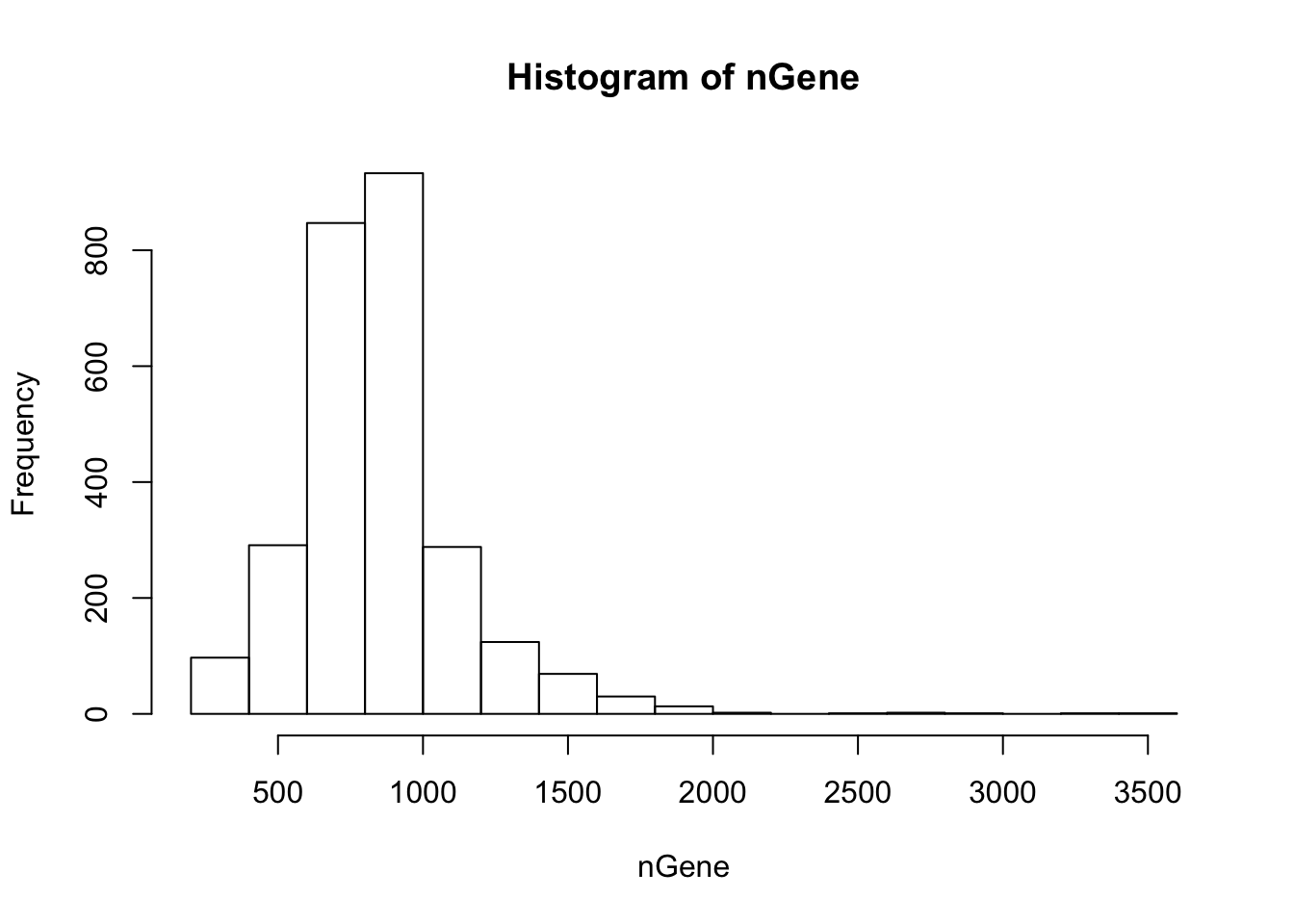
Expand here to see past versions of cell_filter-1.png:
| Version | Author | Date |
|---|---|---|
| f6c8902 | tk382 | 2018-08-29 |
summaryX = cellFilter(X = orig,
                      genenames = orig_genenames$V2,
                      minGene = 500,
                      maxGene = 2000,
                      maxMitoProp = 0.1)
tmpX = summaryX$X
nUMI = summaryX$nUMI
nGene = summaryX$nGene
percent.mito = summaryX$percent.mito
det.rate = summaryX$det.rate

par(mfrow = c(1,4))
boxplot(nUMI, main='nUMI');
boxplot(nGene, main='nGene');
boxplot(percent.mito, main='mitogene prop');
boxplot(det.rate, main='detection rate')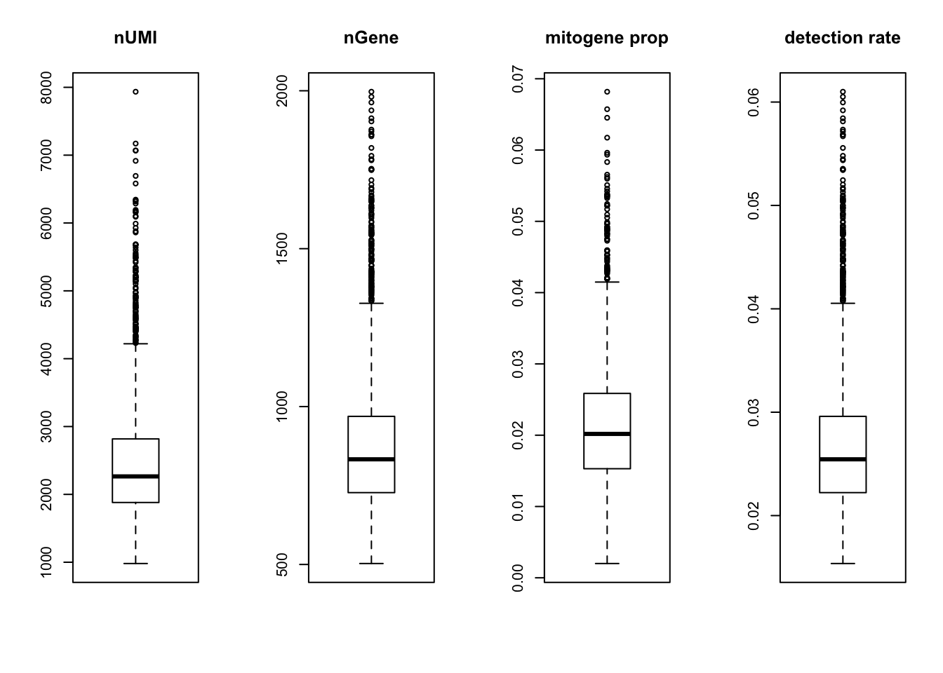
Expand here to see past versions of cell_filter-2.png:
| Version | Author | Date |
|---|---|---|
| f6c8902 | tk382 | 2018-08-29 |
Gene Filtering
Next find variable genes using normalized dispersion. First, remove the genes where counts are 0 in all the cells, so that we use genes with at least one UMI count detected in at least one cell are used. Then genes are placed into a number of bins (user’s choice in “bins” parameter in “dispersion” function, default is 20) based on their mean expression, and normalized dispersion is calculated as the absolute difference between dispersion and median dispersion of the expression mean, normalized by the median absolute deviation within each bin. (Grace Zheng et al., 2017)
X = tmpX[Matrix::rowSums(tmpX) > 0, ]
genenames = orig_genenames[Matrix::rowSums(tmpX) > 0, 2]

disp = dispersion(X, bins = 20, robust = F)

outliers = which(disp$normalized_dispersion>5)
plot(disp$normalized_dispersion[-outliers] ~ disp$genemeans[-outliers],
     xlab = "mean expression",
     ylab = "normalized dispersion",
     ylim = c(min(disp$normalized_dispersion),
              max(disp$normalized_dispersion, na.rm=TRUE)))
text(disp$normalized_dispersion[outliers] ~ disp$genemeans[outliers],
     labels = genenames[outliers],
     cex=0.5)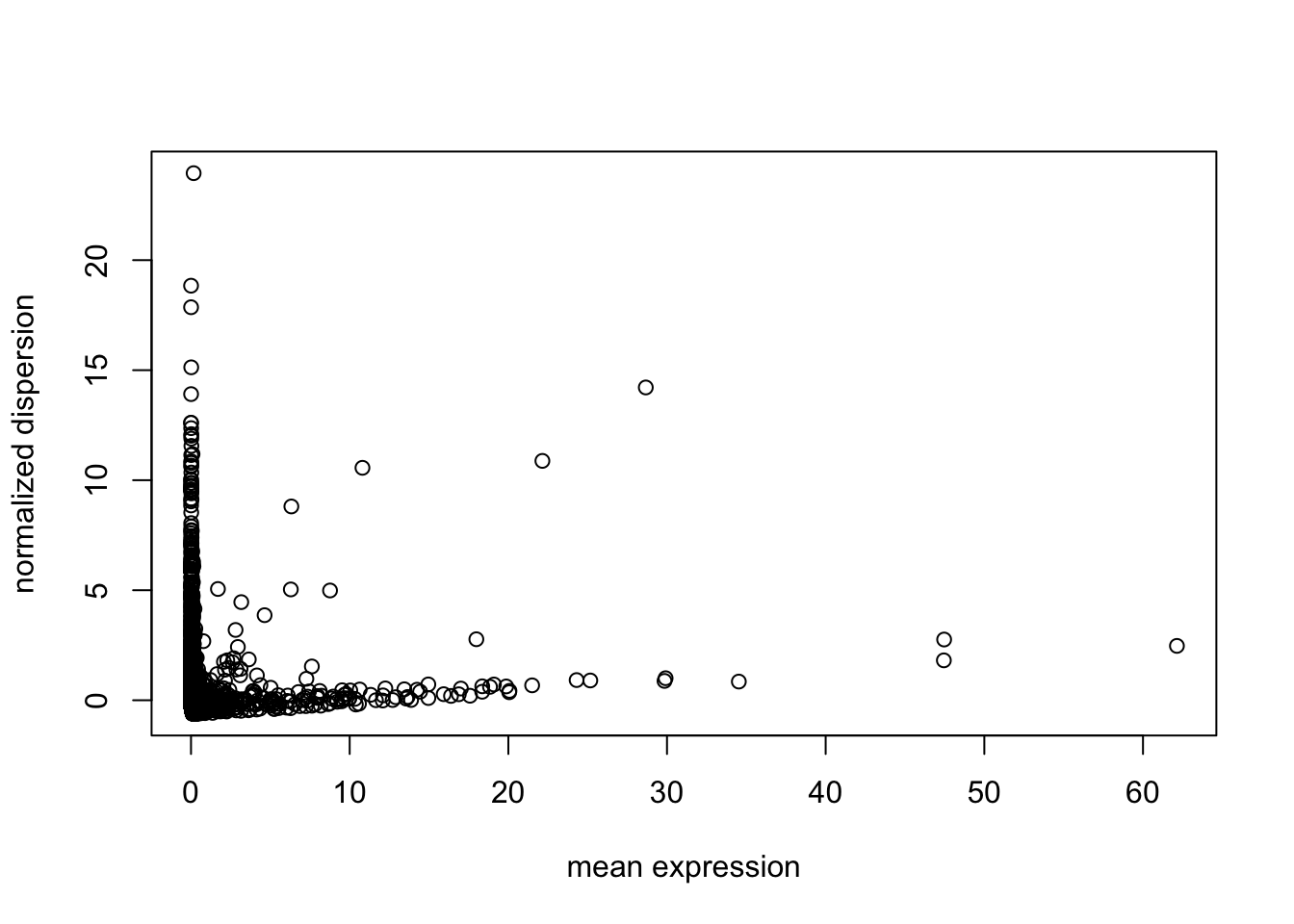
Expand here to see past versions of basic_gene_filtering-1.png:
| Version | Author | Date |
|---|---|---|
| f6c8902 | tk382 | 2018-08-29 |
select = which(abs(disp$normalized_dispersion) > 1)
X = X[select, ]
genenames = genenames[select]
UMI Normalization
Use quantile-normalization to make the distribution of each cell the same.
X = quantile_normalize(as.matrix(X))Dimension reduction and visualization
log.cpm = as.matrix(log(X + 1))
pc.base = irlba(log.cpm, 20)
tsne.base = Rtsne(pc.base$v[,1:10], dims=2, perplexity = 100, pca=FALSE)
rm(pc.base)
plot(tsne.base$Y, cex=0.7, xlab = "tsne1", ylab = "tsne2")
Run SLSL
Run the clustering algorithm SLSL based on the filtered matrix. There are three main parameters. First, “klist” determines the number of neighbors to use to build initial similarity matrix, and around 1/10 of the number of cells is appropriate. “sigmalist” determines the nonlinear structure of Gaussian kernel, and the default of 1, 1.5, and 2.5 work well. The kernel_type determines the distance measure. The four options are “spearman”, “pearson”, “euclidean”, and “combined” which combines information across three different distance measures.
# out = SLSL(log.cpm,
#            klist = c(200,400,600),
#            sigmalist = c(1, 2, 3),
#            kernel_type = "combined",
#            verbose=FALSE)
# tab = table(out$result)
# save(out, file='slsl_10x.Rdata')
load('analysis/slsl_10x.Rdata')
tab = table(out$result)
Analyze result
First visualize the tSNE plot with the clustering result. Also the output includes the similarity matrix that can be visualized using heatmap function, given that there is enough RAM space.
plot(tsne.base$Y, col=rainbow(11)[out$result],
     xlab = 'tsne1', ylab='tsne2', main="SLSL result", cex = 0.5)
S = as.matrix(out$S)

ind = sort(out$result, index.return=TRUE)$ix
Known Markers
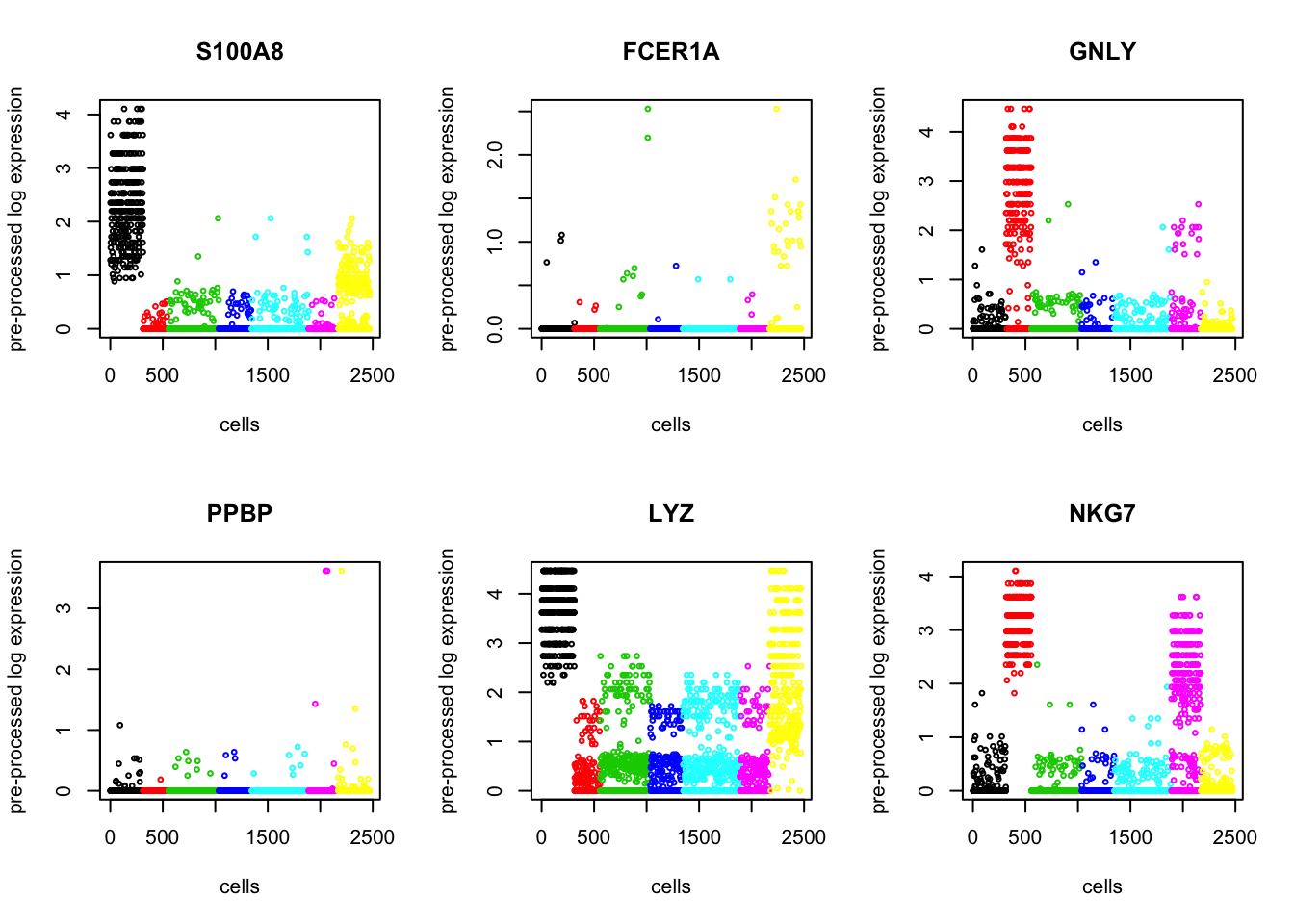
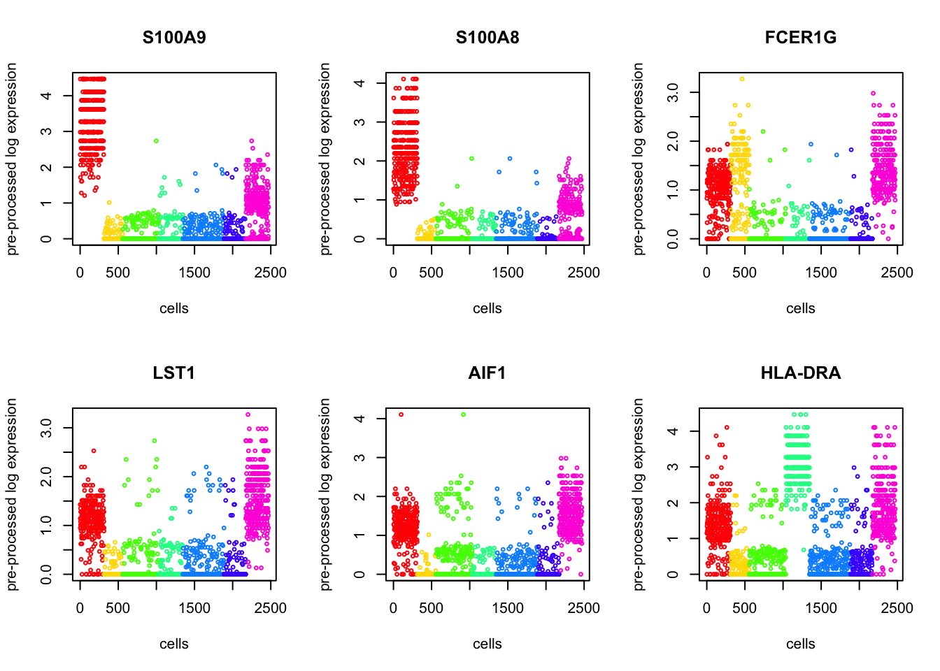
If there are known markers, you can check how differentially they are expressed in the clustering result. The markers used below are from the supplementary table of (Schelker et al., 2017)
sorted_type = sort(out$result, index.return=TRUE)$ix

markers = c('CD3D','CD3E','CD3G','CD27','CD28',
            'CD4',
            'CD8B',
            'CD4','FOXP3','IL2RA','CTLA4',
            'CD19','MS4A1','CD79A','CD79B','BLNK',
            'CD14','CD68','CD163','CSF1R','FCGR3A',
            'IL3RA','CLEC4C','NRP1',
            'FCGR3A','FCGR3B','NCAM1','KLRB1','KLRB1','KLRC1','KLRD1','KLRF1','KLRK1',
            'VWF','CDH5','SELE',
            'FAP','THY1','COL1A1','COL3A1',
            'WFDC2','EPCAM','MCAM',
            'PMEL','MLANA','TYR','MITF'
)
ind = which(orig_genenames$V2 %in% markers)
par(mfrow = c(2,3))
for (i in 1:length(ind)){
  if(sum(tmpX[ind[i], sorted_type]!=0) > 50){
      plot(tmpX[ind[i], sorted_type], col = rainbow(11)[as.factor(out$result[sorted_type])],
       main = orig_genenames[ind[i],2], cex=0.5,
       xlab = 'cells', ylab = 'pre-processed log expression')
  }
}
Expand here to see past versions of biomarkers-1.png:
| Version | Author | Date |
|---|---|---|
| 29d6c3f | tk382 | 2018-08-31 |
| 5cd6432 | tk382 | 2018-08-30 |
| 3018a28 | tk382 | 2018-08-30 |
| f6c8902 | tk382 | 2018-08-29 |

Expand here to see past versions of biomarkers-2.png:
| Version | Author | Date |
|---|---|---|
| 3018a28 | tk382 | 2018-08-30 |


Based on the biomarkers, we can infer that B cells are red, T cells are orange, NK cells are yelow, and monocytes are green.
Differentially Expressed Genes
Using Kruskal test, we order the p-values to find the top differentially expressed genes. Below we present 6.
p = rep(0, nrow(log.cpm))
for (i in 1:nrow(log.cpm)){
  p[i] = kruskal.test(log.cpm[i,], as.factor(out$result))$p.value
}
sorted_p = sort(-log10(p), index.return=TRUE, decreasing = TRUE)
sorted_type = sort(out$result, index.return=TRUE)$ix

par(mfrow = c(2,3))
for (i in 1:6){
  plot(log.cpm[sorted_p$ix[i], sorted_type],
       col = rainbow(11)[as.factor(out$result[sorted_type])],
       main = genenames[sorted_p$ix[i]], cex=0.5,
       ylab = "pre-processed log expression", xlab = "cells")
}
Expand here to see past versions of find_markers-1.png:
| Version | Author | Date |
|---|---|---|
| 29d6c3f | tk382 | 2018-08-31 |
| 5cd6432 | tk382 | 2018-08-30 |
| 3018a28 | tk382 | 2018-08-30 |
Expand here to see past versions of ggplots2-1.png:
| Version | Author | Date |
|---|---|---|
| 29d6c3f | tk382 | 2018-08-31 |
Session information
sessionInfo()R version 3.5.1 (2018-07-02)
Platform: x86_64-apple-darwin15.6.0 (64-bit)
Running under: macOS Sierra 10.12.5
Matrix products: default
BLAS: /Library/Frameworks/R.framework/Versions/3.5/Resources/lib/libRblas.0.dylib
LAPACK: /Library/Frameworks/R.framework/Versions/3.5/Resources/lib/libRlapack.dylib
locale:
[1] en_US.UTF-8/en_US.UTF-8/en_US.UTF-8/C/en_US.UTF-8/en_US.UTF-8
attached base packages:
[1] parallel stats4 stats graphics grDevices utils datasets
[8] methods base
other attached packages:
[1] bindrcpp_0.2.2 gridExtra_2.3
[3] SC3_1.8.0 SingleCellExperiment_1.2.0
[5] SummarizedExperiment_1.10.1 DelayedArray_0.6.2
[7] BiocParallel_1.14.2 Biobase_2.40.0
[9] GenomicRanges_1.32.6 GenomeInfoDb_1.16.0
[11] IRanges_2.14.10 S4Vectors_0.18.3
[13] BiocGenerics_0.26.0 SCNoisyClustering_0.1.0
[15] plotly_4.8.0 gplots_3.0.1
[17] diceR_0.5.1 Rtsne_0.13
[19] igraph_1.2.2 scatterplot3d_0.3-41
[21] pracma_2.1.4 fossil_0.3.7
[23] shapefiles_0.7 foreign_0.8-71
[25] maps_3.3.0 sp_1.3-1
[27] caret_6.0-80 lattice_0.20-35
[29] reshape_0.8.7 dplyr_0.7.6
[31] quadprog_1.5-5 inline_0.3.15
[33] matrixStats_0.54.0 irlba_2.3.2
[35] Matrix_1.2-14 plyr_1.8.4
[37] ggplot2_3.0.0 MultiAssayExperiment_1.6.0
loaded via a namespace (and not attached):
[1] backports_1.1.2 workflowr_1.1.1
[3] lazyeval_0.2.1 splines_3.5.1
[5] digest_0.6.15 foreach_1.4.4
[7] htmltools_0.3.6 gdata_2.18.0
[9] magrittr_1.5 cluster_2.0.7-1
[11] doParallel_1.0.11 ROCR_1.0-7
[13] sfsmisc_1.1-2 recipes_0.1.3
[15] gower_0.1.2 dimRed_0.1.0
[17] R.utils_2.6.0 colorspace_1.3-2
[19] rrcov_1.4-4 WriteXLS_4.0.0
[21] crayon_1.3.4 RCurl_1.95-4.11
[23] jsonlite_1.5 RcppArmadillo_0.8.600.0.0
[25] bindr_0.1.1 survival_2.42-6
[27] iterators_1.0.10 glue_1.3.0
[29] DRR_0.0.3 registry_0.5
[31] gtable_0.2.0 ipred_0.9-6
[33] zlibbioc_1.26.0 XVector_0.20.0
[35] kernlab_0.9-26 ddalpha_1.3.4
[37] DEoptimR_1.0-8 abind_1.4-5
[39] scales_0.5.0 mvtnorm_1.0-8
[41] pheatmap_1.0.10 rngtools_1.3.1
[43] bibtex_0.4.2 Rcpp_0.12.18
[45] viridisLite_0.3.0 xtable_1.8-2
[47] magic_1.5-8 mclust_5.4.1
[49] lava_1.6.2 prodlim_2018.04.18
[51] htmlwidgets_1.2 httr_1.3.1
[53] RColorBrewer_1.1-2 pkgconfig_2.0.1
[55] R.methodsS3_1.7.1 nnet_7.3-12
[57] labeling_0.3 later_0.7.3
[59] tidyselect_0.2.4 rlang_0.2.1
[61] reshape2_1.4.3 munsell_0.5.0
[63] tools_3.5.1 pls_2.6-0
[65] broom_0.5.0 evaluate_0.11
[67] geometry_0.3-6 stringr_1.3.1
[69] yaml_2.2.0 ModelMetrics_1.1.0
[71] knitr_1.20 robustbase_0.93-2
[73] caTools_1.17.1.1 purrr_0.2.5
[75] nlme_3.1-137 doRNG_1.7.1
[77] mime_0.5 whisker_0.3-2
[79] R.oo_1.22.0 RcppRoll_0.3.0
[81] compiler_3.5.1 e1071_1.7-0
[83] tibble_1.4.2 pcaPP_1.9-73
[85] stringi_1.2.4 pillar_1.3.0
[87] data.table_1.11.4 bitops_1.0-6
[89] httpuv_1.4.5 R6_2.2.2
[91] promises_1.0.1 KernSmooth_2.23-15
[93] codetools_0.2-15 MASS_7.3-50
[95] gtools_3.8.1 assertthat_0.2.0
[97] CVST_0.2-2 pkgmaker_0.27
[99] rprojroot_1.3-2 withr_2.1.2
[101] GenomeInfoDbData_1.1.0 grid_3.5.1
[103] rpart_4.1-13 timeDate_3043.102
[105] tidyr_0.8.1 class_7.3-14
[107] rmarkdown_1.10 git2r_0.23.0
[109] shiny_1.1.0 lubridate_1.7.4 This reproducible R Markdown analysis was created with workflowr 1.1.1