Self-organising map (SOM) analysis
Robert Schlegel
2019-06-04
Last updated: 2019-08-01
workflowr checks: (Click a bullet for more information)-
✔ R Markdown file: up-to-date
Great! Since the R Markdown file has been committed to the Git repository, you know the exact version of the code that produced these results.
-
✔ Environment: empty
Great job! The global environment was empty. Objects defined in the global environment can affect the analysis in your R Markdown file in unknown ways. For reproduciblity it’s best to always run the code in an empty environment.
-
✔ Seed:
set.seed(20190513)The command
set.seed(20190513)was run prior to running the code in the R Markdown file. Setting a seed ensures that any results that rely on randomness, e.g. subsampling or permutations, are reproducible. -
✔ Session information: recorded
Great job! Recording the operating system, R version, and package versions is critical for reproducibility.
-
Great! You are using Git for version control. Tracking code development and connecting the code version to the results is critical for reproducibility. The version displayed above was the version of the Git repository at the time these results were generated.✔ Repository version: 5e12d9e
Note that you need to be careful to ensure that all relevant files for the analysis have been committed to Git prior to generating the results (you can usewflow_publishorwflow_git_commit). workflowr only checks the R Markdown file, but you know if there are other scripts or data files that it depends on. Below is the status of the Git repository when the results were generated:
Note that any generated files, e.g. HTML, png, CSS, etc., are not included in this status report because it is ok for generated content to have uncommitted changes.Ignored files: Ignored: .Rhistory Ignored: .Rproj.user/ Ignored: data/ALL_anom.Rda Ignored: data/ERA5_lhf.Rda Ignored: data/ERA5_lwr.Rda Ignored: data/ERA5_qnet.Rda Ignored: data/ERA5_qnet_anom.Rda Ignored: data/ERA5_qnet_clim.Rda Ignored: data/ERA5_shf.Rda Ignored: data/ERA5_swr.Rda Ignored: data/ERA5_t2m.Rda Ignored: data/ERA5_t2m_anom.Rda Ignored: data/ERA5_t2m_clim.Rda Ignored: data/ERA5_u.Rda Ignored: data/ERA5_u_anom.Rda Ignored: data/ERA5_u_clim.Rda Ignored: data/ERA5_v.Rda Ignored: data/ERA5_v_anom.Rda Ignored: data/ERA5_v_clim.Rda Ignored: data/GLORYS_mld.Rda Ignored: data/GLORYS_mld_anom.Rda Ignored: data/GLORYS_mld_clim.Rda Ignored: data/GLORYS_u.Rda Ignored: data/GLORYS_u_anom.Rda Ignored: data/GLORYS_u_clim.Rda Ignored: data/GLORYS_v.Rda Ignored: data/GLORYS_v_anom.Rda Ignored: data/GLORYS_v_clim.Rda Ignored: data/NAPA_clim_U.Rda Ignored: data/NAPA_clim_V.Rda Ignored: data/NAPA_clim_W.Rda Ignored: data/NAPA_clim_emp_ice.Rda Ignored: data/NAPA_clim_emp_oce.Rda Ignored: data/NAPA_clim_fmmflx.Rda Ignored: data/NAPA_clim_mldkz5.Rda Ignored: data/NAPA_clim_mldr10_1.Rda Ignored: data/NAPA_clim_qemp_oce.Rda Ignored: data/NAPA_clim_qla_oce.Rda Ignored: data/NAPA_clim_qns.Rda Ignored: data/NAPA_clim_qsb_oce.Rda Ignored: data/NAPA_clim_qt.Rda Ignored: data/NAPA_clim_runoffs.Rda Ignored: data/NAPA_clim_ssh.Rda Ignored: data/NAPA_clim_sss.Rda Ignored: data/NAPA_clim_sst.Rda Ignored: data/NAPA_clim_taum.Rda Ignored: data/NAPA_clim_vars.Rda Ignored: data/NAPA_clim_vecs.Rda Ignored: data/OAFlux.Rda Ignored: data/OISST_sst.Rda Ignored: data/OISST_sst_anom.Rda Ignored: data/OISST_sst_clim.Rda Ignored: data/node_mean_all_anom.Rda Ignored: data/packet_all.Rda Ignored: data/packet_all_anom.Rda Ignored: data/packet_nolab.Rda Ignored: data/packet_nolab14.Rda Ignored: data/packet_nolabgsl.Rda Ignored: data/packet_nolabmod.Rda Ignored: data/som_all.Rda Ignored: data/som_all_anom.Rda Ignored: data/som_nolab.Rda Ignored: data/som_nolab14.Rda Ignored: data/som_nolab_16.Rda Ignored: data/som_nolab_9.Rda Ignored: data/som_nolabgsl.Rda Ignored: data/som_nolabmod.Rda Ignored: data/synoptic_states.Rda Ignored: data/synoptic_vec_states.Rda Ignored: output/node_summary/
Expand here to see past versions:
| File | Version | Author | Date | Message |
|---|---|---|---|---|
| Rmd | 5e12d9e | robwschlegel | 2019-08-01 | Re-publish entire site. |
| Rmd | 9a9fa7d | robwschlegel | 2019-08-01 | A more in depth dive into the potential criteria to meet for the SOM model |
| Rmd | 240a7a0 | robwschlegel | 2019-07-31 | Ran the base SOM results |
| html | aa82e6e | robwschlegel | 2019-07-31 | Build site. |
| Rmd | 498909b | robwschlegel | 2019-07-31 | Re-publish entire site. |
| html | 35987b4 | robwschlegel | 2019-07-09 | Build site. |
| Rmd | 34efa43 | robwschlegel | 2019-07-09 | Added some thinking to the SOM vignette. |
| html | e2f6f42 | robwschlegel | 2019-07-09 | Build site. |
| Rmd | 609cca8 | robwschlegel | 2019-07-09 | Added some thinking to the SOM vignette. |
| html | 81e961d | robwschlegel | 2019-07-09 | Build site. |
| Rmd | 7ff9b8b | robwschlegel | 2019-06-17 | More work on the talk |
| Rmd | b25762e | robwschlegel | 2019-06-12 | More work on figures |
| Rmd | 413bb8b | robwschlegel | 2019-06-12 | Working on pixel interpolation |
| html | c23c50b | robwschlegel | 2019-06-10 | Build site. |
| html | 028d3cc | robwschlegel | 2019-06-10 | Build site. |
| Rmd | c6b3c7b | robwschlegel | 2019-06-10 | Re-publish entire site. |
| Rmd | 1b53eeb | robwschlegel | 2019-06-10 | SOM packet pipeline testing |
| Rmd | 4504e12 | robwschlegel | 2019-06-07 | Working on joining in vector data |
| html | c61a15f | robwschlegel | 2019-06-06 | Build site. |
| Rmd | 44ac335 | robwschlegel | 2019-06-06 | Working on inclusion of vectors into SOM pipeline |
| html | 6dd6da8 | robwschlegel | 2019-06-06 | Build site. |
| Rmd | 07137d9 | robwschlegel | 2019-06-06 | Site wide update, including newly functioning SOM pipeline. |
| Rmd | 990693a | robwschlegel | 2019-06-05 | First SOM result visuals |
| Rmd | 25e7e9a | robwschlegel | 2019-06-05 | SOM pipeline nearly finished |
| Rmd | 4838cc8 | robwschlegel | 2019-06-04 | Working on SOM functions |
| Rmd | 94ce8f6 | robwschlegel | 2019-06-04 | Functions for creating data packets are up and running |
| Rmd | 65301ed | robwschlegel | 2019-05-30 | Push before getting rid of some testing structure |
| html | c09b4f7 | robwschlegel | 2019-05-24 | Build site. |
| Rmd | 5dc8bd9 | robwschlegel | 2019-05-24 | Finished initial creation of SST prep vignette. |
| html | a29be6b | robwschlegel | 2019-05-13 | Build site. |
| html | ea61999 | robwschlegel | 2019-05-13 | Build site. |
| Rmd | f8f28b1 | robwschlegel | 2019-05-13 | Skeleton files |
Introduction
This vignette contains the code used to perform the self-organising map (SOM) analysis on the mean synoptic states created in the Variable preparation vignette. We’ll start by creating custom packets that meet certain experimental criteria before then feeding them into a SOM. We will finish up by creating some cursory visuals of the results. The full summary of the results may be seen in the Node summary vignette.
# Insatll from GitHub
# .libPaths(c("~/R-packages", .libPaths()))
# devtools::install_github("fabrice-rossi/yasomi")

# Packages used in this vignette
library(jsonlite, lib.loc = "../R-packages/")
library(tidyverse) # Base suite of functions
library(ncdf4) # For opening and working with NetCDF files
library(lubridate) # For convenient date manipulation
# library(scales) # For scaling data before running SOM
library(yasomi, lib.loc = "../R-packages/") # The SOM package of choice due to PCI compliance
library(data.table) # For working with massive dataframes

# Set number of cores
doMC::registerDoMC(cores = 50)

# Disable scientific notation for numeric values
  # I just find it annoying
options(scipen = 999)

# Set number of cores
doMC::registerDoMC(cores = 50)

# Disable scientific notation for numeric values
  # I just find it annoying
options(scipen = 999)

# Individual regions
NWA_coords <- readRDS("data/NWA_coords_cabot.Rda")

# The NAPA variables
NAPA_vars <- readRDS("data/NAPA_vars.Rda")

# Corners of the study area
NWA_corners <- readRDS("data/NWA_corners.Rda")

# The base map
map_base <- ggplot2::fortify(maps::map(fill = TRUE, col = "grey80", plot = FALSE)) %>%
  dplyr::rename(lon = long) %>%
  mutate(group = ifelse(lon > 180, group+9999, group),
         lon = ifelse(lon > 180, lon-360, lon)) %>%
  select(-region, -subregion)

# MHW results
OISST_region_MHW <- readRDS("data/OISST_region_MHW.Rda")

# MHW Events
OISST_MHW_event <- OISST_region_MHW %>%
  select(-cats) %>%
  unnest(events) %>%
  filter(row_number() %% 2 == 0) %>%
  unnest(events)

# MHW Categories
suppressWarnings( # Don't need warning about different names for events
OISST_MHW_cats <- OISST_region_MHW %>%
  select(-events) %>%
  unnest(cats)
)
Tailored data packets
In this last stage before running our SOM analyses we will create data packets that can be fed directly into the SOM algorithm. These data packets will vary based on the exclusion of certain regions in the study area. In the first run of this analysis on the NAPA model data it was found that the inclusion of the Labrador Sea complicated the results quite a bit. It is also unclear whether or not the Gulf of St Lawrence region should be included in the analysis. While creating whatever packets we desire we will also be converting them into the super-wide matrix format that the SOM model desires.
Unnest synoptic state packets
Up first we must simply load and unnest the synoptic state packets made previously.
# Load the synoptic states data packet
system.time(
synoptic_states <- readRDS("data/synoptic_states.Rda")
) # 3 seconds

# Unnest the synoptic data
system.time(
synoptic_states_unnest <- synoptic_states %>%
  select(region, event_no, synoptic) %>%
  unnest()
) # 8 seconds
Custom packets
With all of our data ready we may now trim them as we see fit before saving them for the SOM.
# The study area size when the Labrador region is excluded
NWA_coords_nolab <- NWA_coords %>%
  filter(region != "ls")

# The study area size when the Labrador and GSL regions are excluded
NWA_coords_nolabgsl <- NWA_coords %>%
  filter(!region %in% c("ls", "gsl"))

# Test visuals of reduced study areas
# synoptic_states[1,] %>%
#   unnest() %>%
#   filter(lat <= round(max(NWA_coords_nolabgsl$lat))+0.5) %>%
#   ggplot(aes(x = lon, y = lat)) +
#   geom_raster(aes(fill = sst_anom)) +
#   geom_polygon(data = NWA_coords_nolabgsl, aes(colour = region), fill = NA)

# Function for casting wide the custom packets
create_packet <- function(df){
  # Cast the data to a single row
  res <- data.table::data.table(df) %>%
    reshape2::melt(id = c("region", "event_no", "lon", "lat"),
                   measure = c(colnames(.)[-c(1:4)]),
                   variable.name = "var", value.name = "val") %>%
    dplyr::arrange(var, lon, lat) %>%
    unite(coords, c(lon, lat, var), sep = "BBB") %>%
    unite(event_ID, c(region, event_no), sep = "BBB") %>%
    reshape2::dcast(event_ID ~ coords, value.var = "val")
  # Remove columns (pixels) with missing data
  res_fix <- res[,colSums(is.na(res))<1]
  return(res_fix)
}

# Packet for entire study region
system.time(
  packet_all <- create_packet(synoptic_states_unnest)
) # 185 seconds
# saveRDS(packet_all, "data/packet_all.Rda")

# Exclude Labrador region
system.time(
  packet_nolab <- synoptic_states_unnest %>%
    filter(region != "ls",
           lat <= round(max(NWA_coords_nolab$lat))+0.5) %>%
    create_packet()
) # 142 seconds
# saveRDS(packet_nolab, "data/packet_nolab.Rda")

# Exclude Labrador and Gulf of St Lawrence regions
system.time(
  packet_nolabgsl <- synoptic_states_unnest %>%
    filter(!region %in% c("ls", "gsl"),
           lat <= round(max(NWA_coords_nolabgsl$lat))+0.5) %>%
    create_packet()
) # 106 seconds
# saveRDS(packet_nolabgsl, "data/packet_nolabgsl.Rda")

# Exclude Labrador region and moderate events
system.time(
  packet_nolabmod <- synoptic_states_unnest %>%
    filter(region != "ls",
           lat <= round(max(NWA_coords_nolab$lat))+0.5) %>%
    left_join(select(OISST_MHW_cats, region, event_no, category), by = c("region", "event_no")) %>%
    filter(category != "I Moderate") %>%
    select(-category) %>%
    create_packet()
) # 15 seconds
# saveRDS(packet_nolabmod, "data/packet_nolabmod.Rda")

# Exclude Labrador region and moderate events
system.time(
  packet_nolab14 <- synoptic_states_unnest %>%
    filter(region != "ls",
           lat <= round(max(NWA_coords_nolab$lat))+0.5) %>%
    left_join(select(OISST_MHW_cats, region, event_no, duration), by = c("region", "event_no")) %>%
    filter(duration >= 14) %>%
    select(-duration) %>%
    create_packet()
) # 40 seconds
# saveRDS(packet_nolab14, "data/packet_nolab14.Rda")
Run SOM models
Now that we have our data packets to feed the SOM, we need a function that will ingest them and produce results for us. The function below has been greatly expanded on from the previous version of this project and now performs all of the SOM related work in one go. This allowed me to remove a couple hundreds lines of code and text from this vignette.
# Function for calculating SOMs using PCI
# This outputs the mean values for each SOM as well
  # NB: 4x4 produced one empty cell and one cell with only one event
  # So the default size has been reduced to 4x3
som_model_PCI <- function(data_packet, xdim = 4, ydim = 3){
  # Create a scaled matrix for the SOM
  # Cancel out first column as this is the reference ID of the event per row
  data_packet_matrix <- as.matrix(scale(data_packet[,-1]))

  # Create the grid that the SOM will use to determine the number of nodes
  som_grid <- somgrid(xdim = xdim, ydim = ydim, topo = "hexagonal")

  # Run the SOM with PCI
  som_model <- batchsom(data_packet_matrix,
                        somgrid = som_grid,
                        init = "pca",
                        max.iter = 100)

  # Create a data.frame of info
  node_info <- data.frame(event_ID = data_packet[,"event_ID"],
                           node = som_model$classif) %>%
    separate(event_ID, into = c("region", "event_no"), sep = "BBB") %>%
    group_by(node) %>%
    mutate(count = n()) %>%
    ungroup() %>%
    mutate(event_no = as.numeric(as.character(event_no))) %>%
    left_join(select(OISST_MHW_cats, region, event_no, category, peak_date),
              by = c("region", "event_no")) %>%
    mutate(month_peak = lubridate::month(peak_date, label = T),
           season_peak = case_when(month_peak %in% c("Jan", "Feb", "Mar") ~ "Winter",
                                   month_peak %in% c("Apr", "May", "Jun") ~ "Spring",
                                   month_peak %in% c("Jul", "Aug", "Sep") ~ "Summer",
                                   month_peak %in% c("Oct", "Nov", "Dec") ~ "Autumn")) %>%
    select(-peak_date, -month_peak)

  # Determine which event goes in which node and melt
  data_packet_long <- cbind(node = som_model$classif, data_packet) %>%
    separate(event_ID, into = c("region", "event_no"), sep = "BBB") %>%
    data.table() %>%
    reshape2::melt(id = c("node", "region", "event_no"),
                   measure = c(colnames(.)[-c(1:3)]),
                   variable.name = "variable", value.name = "value")

  # Create the mean values that serve as the unscaled results from the SOM
  node_data <- data_packet_long[, .(val = mean(value, na.rm = TRUE)),
                                   by = .(node, variable)] %>%
    separate(variable, into = c("lon", "lat", "var"), sep = "BBB") %>%
    dplyr::arrange(node, var, lon, lat) %>%
    mutate(lon = as.numeric(lon),
           lat = as.numeric(lat),
           val = round(val, 4))

  ## ANOSIM for goodness of fit for node count
  node_data_wide <- node_data %>%
    unite(coords, c(lon, lat, var), sep = "BBB") %>%
    data.table() %>%
    dcast(node~coords, value.var = "val")

  # Calculate similarity
  som_anosim <- vegan::anosim(as.matrix(node_data_wide[,-1]),
                              node_data_wide$node, distance = "euclidean")$signif

  # Combine and exit
  res <- list(data = node_data, info = node_info, ANOSIM = paste0("p = ",som_anosim))
  return(res)
}
With the function sorted, we now feed it the data packets.
# The SOM on the entire study area
packet_all <- readRDS("data/packet_all.Rda")
system.time(som_all <- som_model_PCI(packet_all)) # 136 seconds
som_all$ANOSIM # p = 0.001
saveRDS(som_all, file = "data/som_all.Rda")

# The SOM excluding the Labrador Sea region
packet_nolab <- readRDS("data/packet_nolab.Rda")
system.time(som_nolab <- som_model_PCI(packet_nolab)) # 72 seconds
som_nolab$ANOSIM # p = 0.001
saveRDS(som_nolab, file = "data/som_nolab.Rda")

# The SOM excluding the Labrador Sea and Gulf of St Lawrence regions
packet_nolabgsl <- readRDS("data/packet_nolabgsl.Rda")
system.time(som_nolabgsl <- som_model_PCI(packet_nolabgsl)) # 58 seconds
som_nolabgsl$ANOSIM # p = 0.001
saveRDS(som_nolabgsl, file = "data/som_nolabgsl.Rda")

# We see below that the results are crisper when we leave the Gulf of St Lawrence in,
# so we will proceed with the rest of the experiments only excluding the Labrador Shelf

# A 9 node SOM
system.time(som_nolab_9 <- som_model_PCI(packet_nolab, xdim = 3,  ydim = 3)) # 56 seconds
som_nolab_9$ANOSIM # p = 0.001
saveRDS(som_nolab_9, file = "data/som_nolab_9.Rda")

# The 9 node results are perhaps easier to make sense of than 12 nodes, but it's not certain

# A 16 node SOM
system.time(som_nolab_16 <- som_model_PCI(packet_nolab, xdim = 4, ydim = 4)) # 91 seconds
som_nolab_16$ANOSIM # p = 0.001
saveRDS(som_nolab_16, file = "data/som_nolab_16.Rda")

# 16 nodes seems unnecessary...

# A SOM without moderate events
system.time(som_nolabmod <- som_model_PCI(packet_nolabmod, xdim = 2, ydim = 2)) # 12 seconds
som_nolabmod$ANOSIM # p = 0.042
saveRDS(som_nolabmod, file = "data/som_nolabmod.Rda")

# There are fewer than 40 category "II Strong" and larger MHWs so using more than 4 nodes wouldn't be appropriate
# These results are defintely too sparse to use for a publication

# A SOM without events shorter than 14 days
system.time(som_nolab14 <- som_model_PCI(packet_nolab14, xdim = 3, ydim = 3)) # 12 seconds
som_nolab14$ANOSIM # p = 0.001
saveRDS(som_nolab14, file = "data/som_nolab14.Rda")
Visualise SOM results
First up the functions for visualising the unpacked results.
# Ease of life function
som_node_visualise <- function(sub_var, som_result,
                               col_num = 4, file_suffix = "",
                               fig_height = 9, fig_width = 13){

  # Subset data
  som_result_sub <- som_result$data %>%
    filter(var == sub_var)

  # Create plot
  som_panel_plot <- ggplot(som_result_sub, aes(x = lon, y = lat)) +
    # geom_point(aes(colour = val)) +
    geom_raster(aes(fill = val)) +
    geom_polygon(data = map_base, aes(group = group), show.legend = F) +
    geom_label(data = som_result$info, aes(x = -60, y = 35, label = paste0("n = ",count))) +
    # geom_polygon(data = NWA_coords, aes(group = region, fill = region, colour = region), alpha = 0.1) +
    coord_cartesian(xlim = c(min(som_result_sub$lon), max(som_result_sub$lon)),
                    ylim = c(min(som_result_sub$lat), max(som_result_sub$lat)),
                    expand = F) +
    scale_fill_gradient2(low = "blue", high = "red") +
    # scale_colour_viridis_c(option = viridis_option) +
    labs(x = NULL, y = NULL, fill = sub_var) +
    facet_wrap(~node, ncol = col_num) +
    theme(legend.position = "bottom")

  # Save and exit
  ggsave(som_panel_plot, filename = paste0("output/SOM_nodes/som_plot_",sub_var,file_suffix,".pdf"),
         height = fig_height, width = fig_width)
  return(som_panel_plot)
}

# Wrapper function to run through all variables at once
som_node_visualise_all <- function(som_base,
                                   col_num = 4, file_suffix = "",
                                   fig_height = 9, fig_width = 13){
  var_list <- unique(som_result$data$var)
  plyr::l_ply(.data = var_list, .fun = som_node_visualise,
              .parallel = T, som_result = som_base,
              col_num = col_num, file_suffix = file_suffix,
              fig_height = fig_height, fig_width = fig_height)
}
And now we create PDFs for each of the variables for each of the nodes for our different conditions.
# No Labrador Shelf
som_node_visualise_all(som_nolab, file_suffix = "_nolab")

# Na Lab or GSL
som_node_visualise_all(som_nolabgsl, file_suffix = "_nogsl")

# Na Lab, 9 nodes
som_node_visualise_all(som_nolab_9, file_suffix = "_9", fig_width = 10, col_num = 3)

# Na Lab, 16 nodes
som_node_visualise_all(som_nolab_16, file_suffix = "_16", fig_height = 12)

# Na Lab and no moderate events
som_node_visualise_all(som_nolabmod, file_suffix = "_nomod", fig_width = 7, fig_height = 6, col_num = 2)

# Na Lab and no events shorter than 14 days
som_node_visualise_all(som_nolab14, file_suffix = "_nolab14", fig_width = 10, col_num = 3)
Juggling back and forth between the SST anomaly photos with and without the Gulf of St Lawrence it first appears that they are very different, but this is mostly due to the top and bottom rows of nodes being flipped. The actual differences are much more muted and the patterns tend to hold. The patterns appear more crisp in the larger of the two study extents. This is likely because the inclusion of the shallow GSL gives more power to the atmospheric variables to compete with the Gulf Stream. For this reason we are going to proceed with the inclusion of the Gulf of St Lawrence.
Looking at different counts of nodes it appears as though 9 is not enough. When 12 nodes are used more detail comes through. Going up to 16 nodes appear to be too much as not much more detail comes through while creating the complexity of more node results to sift through. When the moderate events are removed we are left with only 37 events (synoptic states) to feed the SOM. This means we shouldn’t use more than 4 nodes so as not to (be just shy of) at least 10 potential values binned into each node. The four nodes that are output do show the most clear difference in patterns and actually do a surprising job of ecapsulating the different potential drivers of MHWs. An ANOSIM test on the nodes show that they are different with a p = 0.046. All of the other results have a ANOSIM of p = 0.001. One issue with screening the events by category is that this part of the ocean experiences many long category I Moderate events that may still be relevant.
So rather than screen by category, I also made a run on the SOM with MHW data with events shorter than 14 days removed. This left us with 103 events to work with, whcih is a good number to use with a 3x3 grid. The results tell perhaps a clearer story than with the 12 nodes and all MHWs.
Just from looking at the node summaries created in this vignette it is too difficult to say conclusively which conditional produces the clearest results. We will need to proceed with the creation of the more in depth node summary figures in order to get a better idea of how well this is working out. Also unresolved in this vignette is the criticism that the methodology used for the creation of the mean synoptic states fed to the SOM is weak to long events coming through as “grey”, meaning they average out to a rather unremarkable state, even though they are likely the most important of all. One proposed fix for this is to create synoptic states using only the peak date of the event, rather than a mean over the range of the event. This should be looked into…
A last point here is also that this methodology should also be useful for looking backwards and forwards through time to see what the synoptic states looked like leading up to and just after the event. This information could be more useful than the first wave of results. Before doing this however a singular methodology needs to be pinned down (i.e. which events to screen and how many nodes to use).
See the files in the /output/SOM_nodes/ folder in the GitHub repo for this project. They aren’t all shown here because they take a bit too long to render. But the following shows what the SST anomaly nodes look like.
plot_sst_anom <- som_node_visualise(sub_var = "sst_anom", som_result = som_nolab)
plot_sst_anom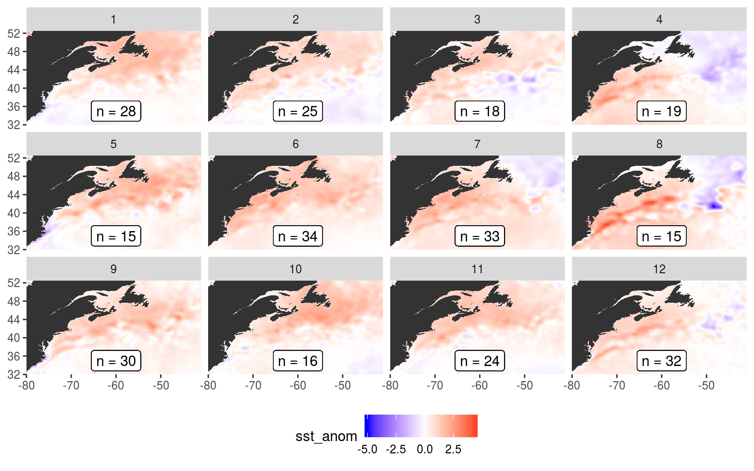
Expand here to see past versions of plot-sst-anom-1.png:
| Version | Author | Date |
|---|---|---|
| aa82e6e | robwschlegel | 2019-07-31 |
| 81e961d | robwschlegel | 2019-07-09 |
| 028d3cc | robwschlegel | 2019-06-10 |
Up next in the Node summary vignette we will show the results in more depth. The code used to create the summary figures may be found in the Figures vignette.
Musings
Possible mechanisms
“Finally, Shearman and Lentz (2010) showed that century-long ocean warming trends observed along the entire northeast U.S. coast are not related to local atmospheric forcing but driven by atmospheric warming of source waters in the Labrador Sea and the Arctic, which are advected into the region.” (Richaud et al., 2016)
Downwelling
Net heatflux (OAFlux) doesn’t line up perfectly with seasonal SST signal, but is very close, with heat flux tending to lead SST by 2 – 3 months (Richaud et al., 2016). It is therefore likely one of the primary drivers of SST and should therefore be strongly considered when constructing SOMs.
There is almost no seasonal cycle for slope waters in any of the regions (Richaud et al., 2016).
More ideas
It would be interesting to see if the SOM outputs differ in any meaningful ways when only data from the first half of the study time period are used compared against the second half.
The output of the SOMs could likely be more meaningfully conveyed from the point of view of the regions. What I mean by this is to take the summary of the nodes, convey them into a table, and then use that table to inform a series of information bits that is focused around each region. Some sort of interactive visual may be useful for this. Showing the percentage that each region has in each node would be a good start. This would allow for a more meaningful further explanation for which drivers affect which regions during which seasons and over which years.
Once this summary is worked out it would then follow that the same analysis be run 1, 2, 3 etc. months in the past and see what the same information format provides w.r.t. a sort of predictive capacity. All of this can then be used to check other data products with a more focused lens in order to maximise the utility of the output.
References
Richaud, B., Kwon, Y.-O., Joyce, T. M., Fratantoni, P. S., and Lentz, S. J. (2016). Surface and bottom temperature and salinity climatology along the continental shelf off the canadian and us east coasts. Continental Shelf Research 124, 165–181.
Session information
sessionInfo()R version 3.6.1 (2019-07-05)
Platform: x86_64-pc-linux-gnu (64-bit)
Running under: Ubuntu 16.04.5 LTS
Matrix products: default
BLAS: /usr/lib/openblas-base/libblas.so.3
LAPACK: /usr/lib/libopenblasp-r0.2.18.so
locale:
[1] LC_CTYPE=en_CA.UTF-8 LC_NUMERIC=C
[3] LC_TIME=en_CA.UTF-8 LC_COLLATE=en_CA.UTF-8
[5] LC_MONETARY=en_CA.UTF-8 LC_MESSAGES=en_CA.UTF-8
[7] LC_PAPER=en_CA.UTF-8 LC_NAME=C
[9] LC_ADDRESS=C LC_TELEPHONE=C
[11] LC_MEASUREMENT=en_CA.UTF-8 LC_IDENTIFICATION=C
attached base packages:
[1] stats graphics grDevices utils datasets methods base
other attached packages:
[1] bindrcpp_0.2.2 data.table_1.11.6 yasomi_0.3
[4] proxy_0.4-22 e1071_1.7-0 lubridate_1.7.4
[7] ncdf4_1.16 forcats_0.3.0 stringr_1.3.1
[10] dplyr_0.7.6 purrr_0.2.5 readr_1.1.1
[13] tidyr_0.8.1 tibble_1.4.2 ggplot2_3.0.0
[16] tidyverse_1.2.1 jsonlite_1.6
loaded via a namespace (and not attached):
[1] tidyselect_0.2.4 haven_1.1.2 lattice_0.20-35
[4] colorspace_1.3-2 htmltools_0.3.6 yaml_2.2.0
[7] rlang_0.2.2 R.oo_1.22.0 pillar_1.3.0
[10] glue_1.3.0 withr_2.1.2 R.utils_2.7.0
[13] doMC_1.3.5 modelr_0.1.2 readxl_1.1.0
[16] foreach_1.4.4 bindr_0.1.1 plyr_1.8.4
[19] munsell_0.5.0 gtable_0.2.0 workflowr_1.1.1
[22] cellranger_1.1.0 rvest_0.3.2 R.methodsS3_1.7.1
[25] codetools_0.2-15 evaluate_0.11 labeling_0.3
[28] knitr_1.20 parallel_3.6.1 class_7.3-14
[31] broom_0.5.0 Rcpp_0.12.18 backports_1.1.2
[34] scales_1.0.0 hms_0.4.2 digest_0.6.16
[37] stringi_1.2.4 grid_3.6.1 rprojroot_1.3-2
[40] cli_1.0.0 tools_3.6.1 maps_3.3.0
[43] magrittr_1.5 lazyeval_0.2.1 crayon_1.3.4
[46] whisker_0.3-2 pkgconfig_2.0.2 xml2_1.2.0
[49] iterators_1.0.10 assertthat_0.2.0 rmarkdown_1.10
[52] httr_1.3.1 rstudioapi_0.7 R6_2.2.2
[55] nlme_3.1-137 git2r_0.23.0 compiler_3.6.1 This reproducible R Markdown analysis was created with workflowr 1.1.1