Node summary
Robert Schlegel
2019-07-09
Last updated: 2019-08-11
workflowr checks: (Click a bullet for more information)-
✔ R Markdown file: up-to-date
Great! Since the R Markdown file has been committed to the Git repository, you know the exact version of the code that produced these results.
-
✔ Environment: empty
Great job! The global environment was empty. Objects defined in the global environment can affect the analysis in your R Markdown file in unknown ways. For reproduciblity it’s best to always run the code in an empty environment.
-
✔ Seed:
set.seed(20190513)The command
set.seed(20190513)was run prior to running the code in the R Markdown file. Setting a seed ensures that any results that rely on randomness, e.g. subsampling or permutations, are reproducible. -
✔ Session information: recorded
Great job! Recording the operating system, R version, and package versions is critical for reproducibility.
-
Great! You are using Git for version control. Tracking code development and connecting the code version to the results is critical for reproducibility. The version displayed above was the version of the Git repository at the time these results were generated.✔ Repository version: d46e344
Note that you need to be careful to ensure that all relevant files for the analysis have been committed to Git prior to generating the results (you can usewflow_publishorwflow_git_commit). workflowr only checks the R Markdown file, but you know if there are other scripts or data files that it depends on. Below is the status of the Git repository when the results were generated:
Note that any generated files, e.g. HTML, png, CSS, etc., are not included in this status report because it is ok for generated content to have uncommitted changes.Ignored files: Ignored: .Rhistory Ignored: .Rproj.user/ Ignored: data/ALL_anom.Rda Ignored: data/ALL_clim.Rda Ignored: data/ERA5_lhf.Rda Ignored: data/ERA5_lwr.Rda Ignored: data/ERA5_qnet.Rda Ignored: data/ERA5_qnet_anom.Rda Ignored: data/ERA5_qnet_clim.Rda Ignored: data/ERA5_shf.Rda Ignored: data/ERA5_swr.Rda Ignored: data/ERA5_t2m.Rda Ignored: data/ERA5_t2m_anom.Rda Ignored: data/ERA5_t2m_clim.Rda Ignored: data/ERA5_u.Rda Ignored: data/ERA5_u_anom.Rda Ignored: data/ERA5_u_clim.Rda Ignored: data/ERA5_v.Rda Ignored: data/ERA5_v_anom.Rda Ignored: data/ERA5_v_clim.Rda Ignored: data/GLORYS_mld.Rda Ignored: data/GLORYS_mld_anom.Rda Ignored: data/GLORYS_mld_clim.Rda Ignored: data/GLORYS_u.Rda Ignored: data/GLORYS_u_anom.Rda Ignored: data/GLORYS_u_clim.Rda Ignored: data/GLORYS_v.Rda Ignored: data/GLORYS_v_anom.Rda Ignored: data/GLORYS_v_clim.Rda Ignored: data/NAPA_clim_U.Rda Ignored: data/NAPA_clim_V.Rda Ignored: data/NAPA_clim_W.Rda Ignored: data/NAPA_clim_emp_ice.Rda Ignored: data/NAPA_clim_emp_oce.Rda Ignored: data/NAPA_clim_fmmflx.Rda Ignored: data/NAPA_clim_mldkz5.Rda Ignored: data/NAPA_clim_mldr10_1.Rda Ignored: data/NAPA_clim_qemp_oce.Rda Ignored: data/NAPA_clim_qla_oce.Rda Ignored: data/NAPA_clim_qns.Rda Ignored: data/NAPA_clim_qsb_oce.Rda Ignored: data/NAPA_clim_qt.Rda Ignored: data/NAPA_clim_runoffs.Rda Ignored: data/NAPA_clim_ssh.Rda Ignored: data/NAPA_clim_sss.Rda Ignored: data/NAPA_clim_sst.Rda Ignored: data/NAPA_clim_taum.Rda Ignored: data/NAPA_clim_vars.Rda Ignored: data/NAPA_clim_vecs.Rda Ignored: data/OAFlux.Rda Ignored: data/OISST_sst.Rda Ignored: data/OISST_sst_anom.Rda Ignored: data/OISST_sst_clim.Rda Ignored: data/node_mean_all_anom.Rda Ignored: data/packet_all.Rda Ignored: data/packet_all_anom.Rda Ignored: data/packet_nolab.Rda Ignored: data/packet_nolab14.Rda Ignored: data/packet_nolabgsl.Rda Ignored: data/packet_nolabmod.Rda Ignored: data/som_all.Rda Ignored: data/som_all_anom.Rda Ignored: data/som_nolab.Rda Ignored: data/som_nolab14.Rda Ignored: data/som_nolab_16.Rda Ignored: data/som_nolab_9.Rda Ignored: data/som_nolabgsl.Rda Ignored: data/som_nolabmod.Rda Ignored: data/synoptic_states.Rda Ignored: data/synoptic_vec_states.Rda
Expand here to see past versions:
| File | Version | Author | Date | Message |
|---|---|---|---|---|
| Rmd | d46e344 | robwschlegel | 2019-08-11 | Re-publish entire site. |
| html | 19bea26 | robwschlegel | 2019-08-11 | Build site. |
| Rmd | b6e2cd9 | robwschlegel | 2019-08-11 | Re-publish entire site. |
| html | 2652a3a | robwschlegel | 2019-08-11 | Build site. |
| Rmd | 75c138c | robwschlegel | 2019-08-11 | Re-publish entire site. |
| Rmd | adc762b | robwschlegel | 2019-08-08 | Re-worked the GLORYS data and propogated update through to SOM analysis figures for all experiments |
| html | f0d2efb | robwschlegel | 2019-08-07 | Build site. |
| Rmd | 9d81722 | robwschlegel | 2019-08-07 | Re-publish entire site. |
| Rmd | ed626bf | robwschlegel | 2019-08-07 | Ran a bunch of figures and had a meeting with Eric. More changes coming to GLORYS data tomorrow before settling on one of the experimental SOMs |
| html | d4ba012 | robwschlegel | 2019-07-09 | Build site. |
| Rmd | c8a5a1a | robwschlegel | 2019-07-09 | Fixing figure display in vignette. |
| Rmd | 3a740c2 | robwschlegel | 2019-07-09 | Creating assets folder for displaying figures created in other vignettes in new vignettes etc. |
| html | 3a740c2 | robwschlegel | 2019-07-09 | Creating assets folder for displaying figures created in other vignettes in new vignettes etc. |
| html | 81e961d | robwschlegel | 2019-07-09 | Build site. |
| Rmd | 497eeb2 | robwschlegel | 2019-07-09 | Re-publish entire site. |
| Rmd | 95a168d | robwschlegel | 2019-07-09 | Frame of node summary vignette worked out |
Introduction
This vignette will show the summary figures for the various SOM experiments. The code used to create these summary figures may be found in code/functions.R and a more detailed overview is given in the Figures vignette. The SOM experiments are given below by name and abbreviation. Within each experiment, the individual nodes are listed below by their number. Use the table of contents on the left of the screen to move quickly between SOM experiments and their nodes of interest as desired.
Visualise SOM results
With the following lines of code we create PDFs for each of the variables for each of the nodes for our different conditions. These PDFs may be seen at output/SOM/*, where * is the code name denoting which SOM experiment was conducted.
Juggling back and forth between the SST anomaly figures with and without the Gulf of St Lawrence it first appears that they are very different, but this is mostly due to the top and bottom rows of nodes being flipped. The actual differences are much more muted and the patterns tend to hold. The patterns appear more crisp in the larger of the two study extents. This is likely because the inclusion of the shallow GSL gives more power to the atmospheric variables to compete with the Gulf Stream. For this reason we are going to proceed with the inclusion of the Gulf of St Lawrence.
Looking at different counts of nodes it appears as though 9 may not be enough. When 12 nodes are used more detail comes through. Going up to 16 nodes appear to be too much as not much more detail comes through while creating the complexity of more node results to sift through. When the moderate events are removed we are left with only 37 events (synoptic states) to feed the SOM. This means we shouldn’t use more than 4 nodes so as not to (be just shy of) at least 10 potential values binned into each node. The four nodes that are output do show the most clear difference in patterns and actually do a surprising job of encapsulating the different potential drivers of MHWs. An ANOSIM test on the nodes show that they are different with a p = 0.046. All of the other results have a ANOSIM of p = 0.001. One issue with screening the events by category is that this part of the ocean experiences many long category I Moderate events that may still be relevant.
So rather than screen by category, I also made a run on the SOM with MHW data with events shorter than 14 days removed. This left us with 103 events to work with, which is a good number to use with a 3x3 grid. The results tell perhaps a clearer story than with the 12 nodes and all MHWs.
Just from going over the node summaries created in this vignette it is too difficult to say conclusively which SOM experiment produces the clearest results. We will need to go over the summary figures in much more detail in order to get a better idea of how well this is working out. Also unresolved in this vignette is the criticism that the methodology used for the creation of the mean synoptic states fed to the SOM is weak to long events coming through as “grey”, meaning they average out to a rather unremarkable state, even though they are likely the most important of all. One proposed fix for this is to create synoptic states using only the peak date of the event, rather than a mean over the range of the event. This should be looked into…
A last point here is that this methodology should also be useful for looking backwards and forwards through time to see what the synoptic states looked like leading up to and just after the event. This information could be more useful than the first wave of results. Before doing this however a singular methodology needs to be pinned down (i.e. which events to screen and how many nodes to use).
See the files in the /output/SOM_nodes/ folder in the GitHub repo for this project. They aren’t all shown here because they take a bit too long to render.
Figure caption key
The captions for the figures below have a lot of acronyms in them but they are consistently used and I will provide a list of what they are here. Whenever one sees an acronym in lower case letters it is referring to one of the regions of the study area as seen in the following figure.
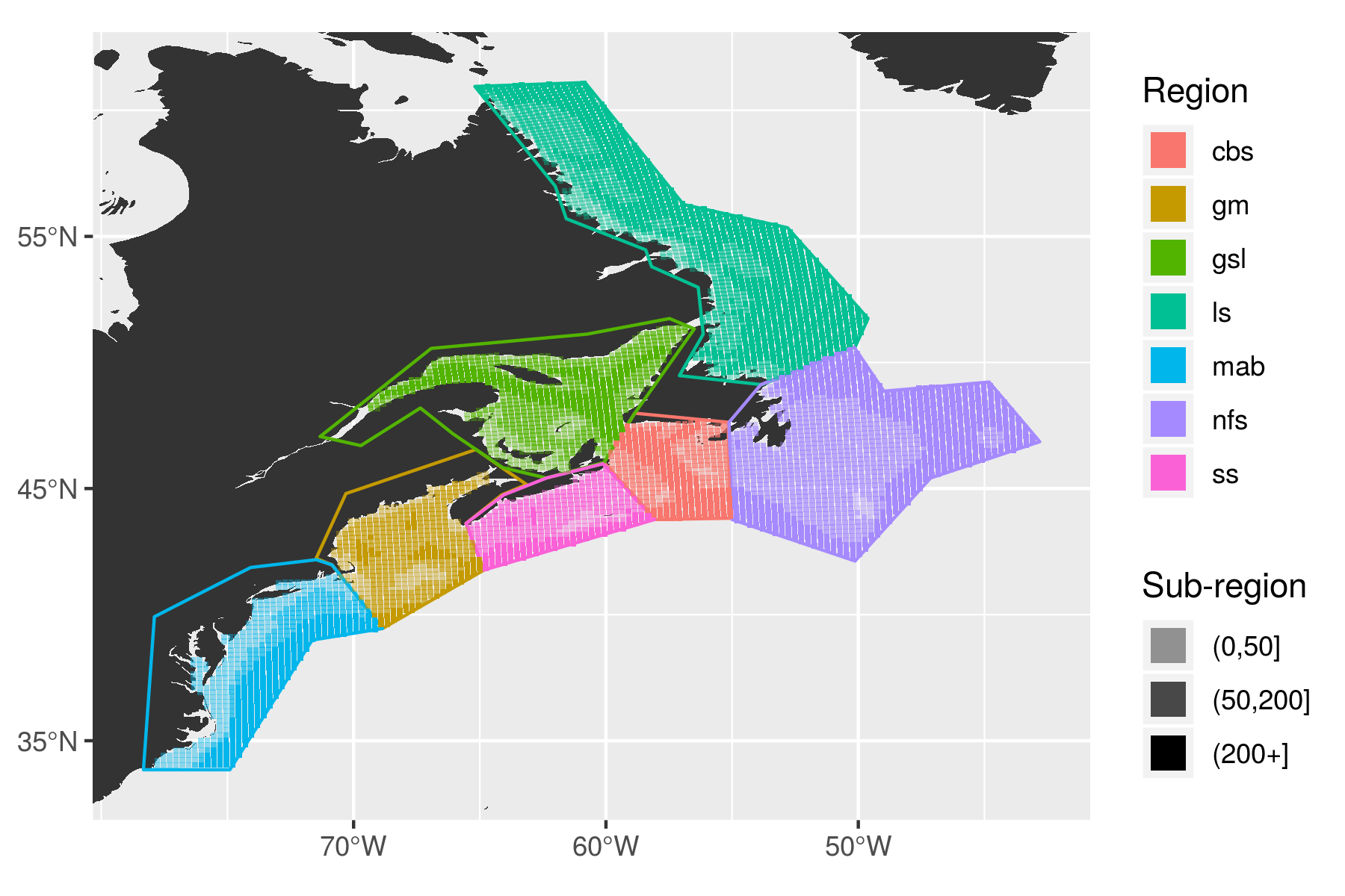
The regions of the coast were devided up by their temperature and salinity regimes based on work by Richaud et al. (2016). The regions were furthered divided into sub-regions based on their depth.
Expand here to see past versions of study_regions.png:
| Version | Author | Date |
|---|---|---|
| 9273f18 | robwschlegel | 2019-08-11 |
The region abbreviations are:
- gm = Gulf of Maine
- gls = Gulf of St. Lawrence
- ls = Labrador Shelf
- mab = Mid-Atlantic Bight
- nfs = Newfoundland Shelf
- ss = Scotian Shelf
The upper case acronyms used in the following figure captions are as follows:
- SST = Sea surface temperature
- SOM = Self-organising map(s)
- GS = Gulf Stream
- AO = Atlantic Ocean
- LS = Labrador Sea
- LC = Labrador Current
- NS = Nova Scotia
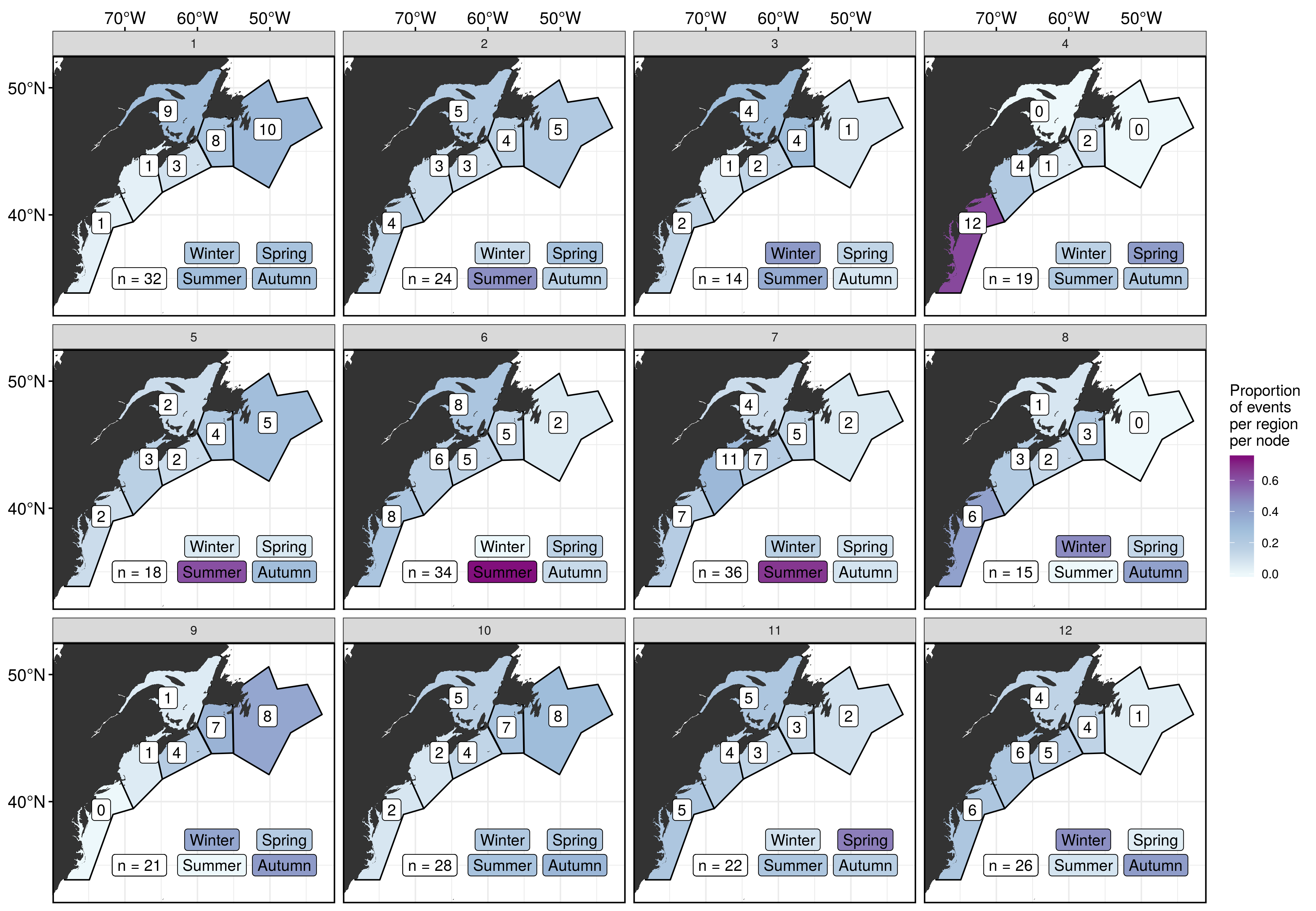
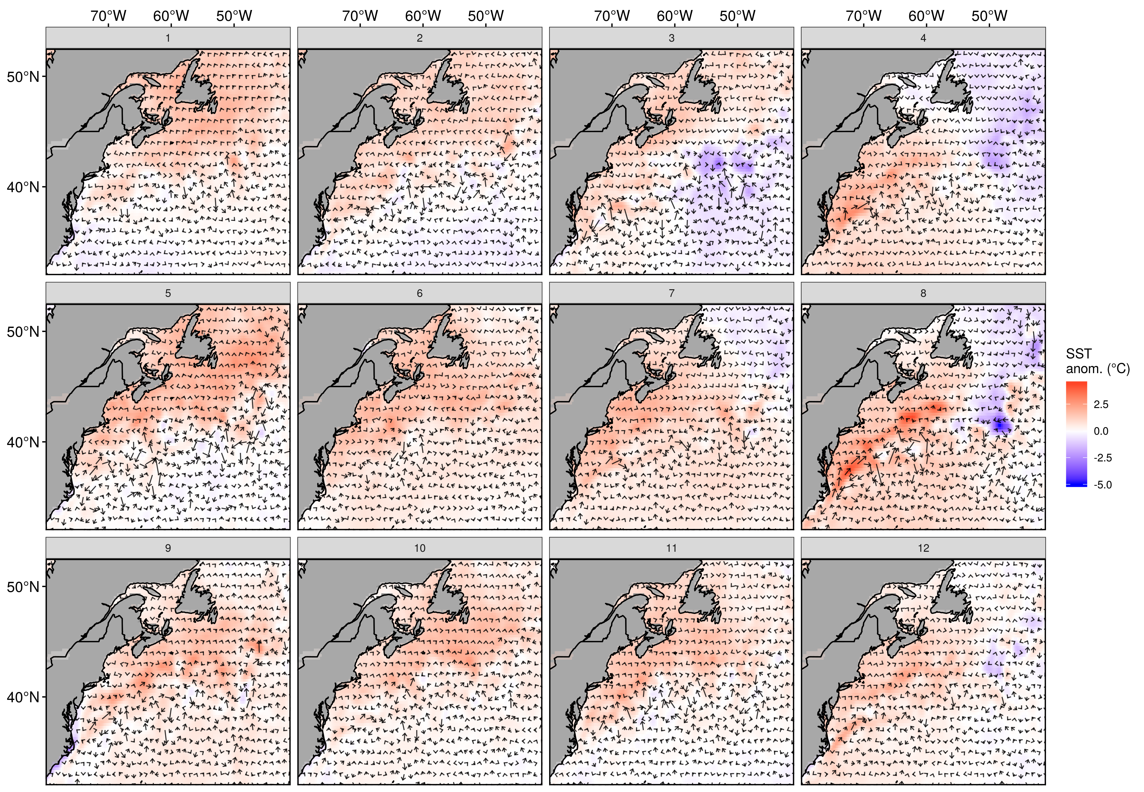
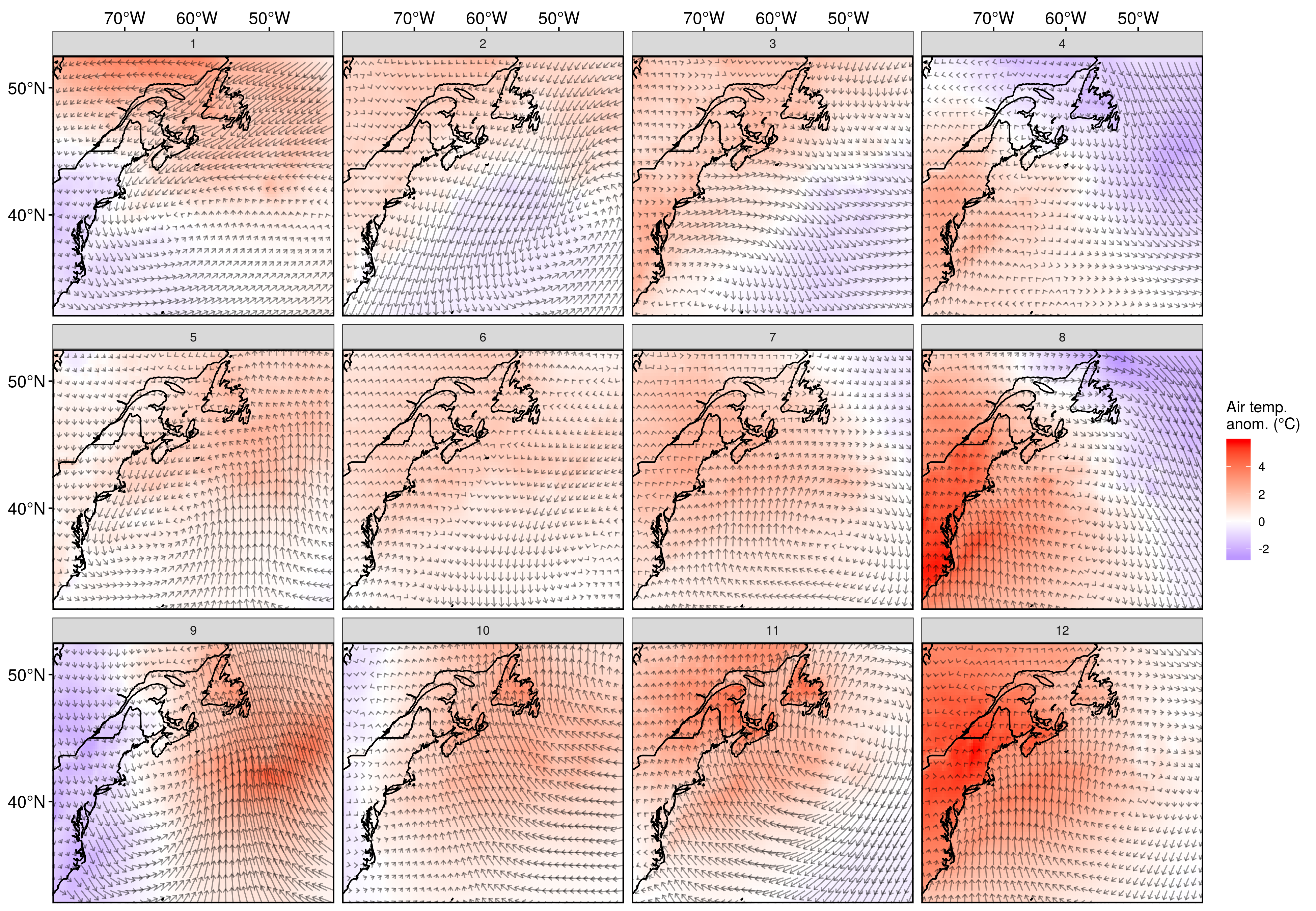
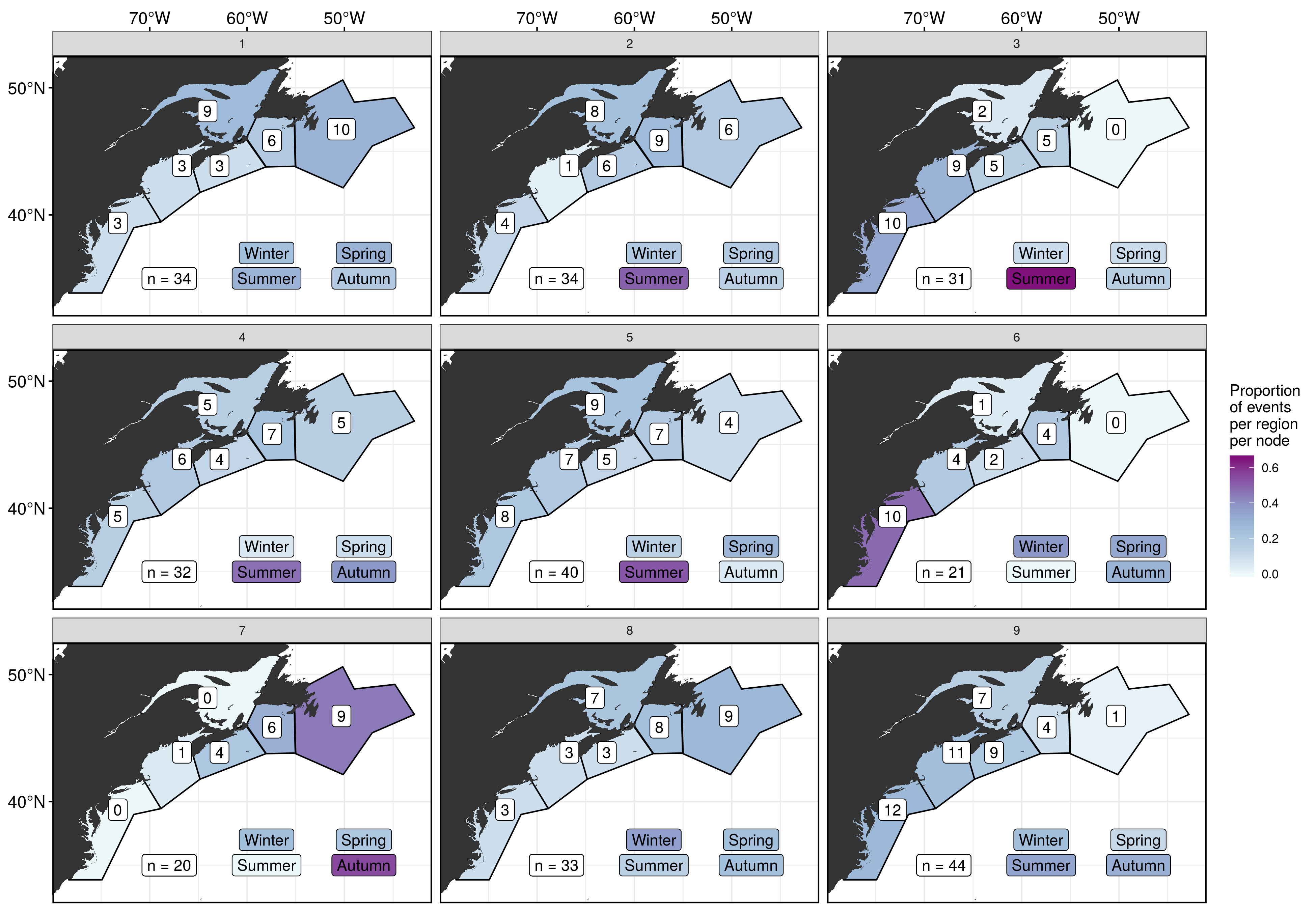
SOM experiment: No Labrador Shelf region (default), 4x3 nodes
Node summary table
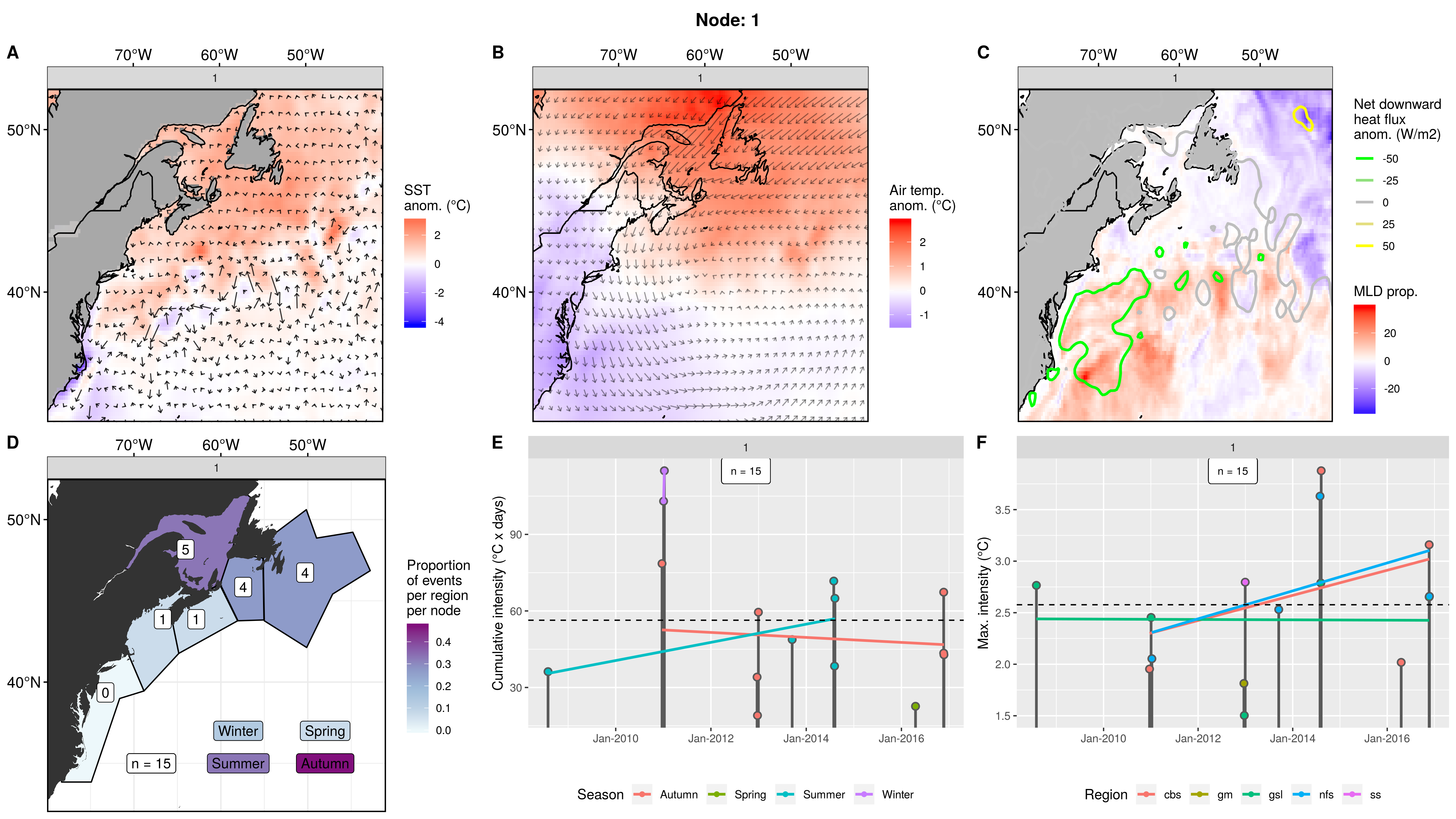
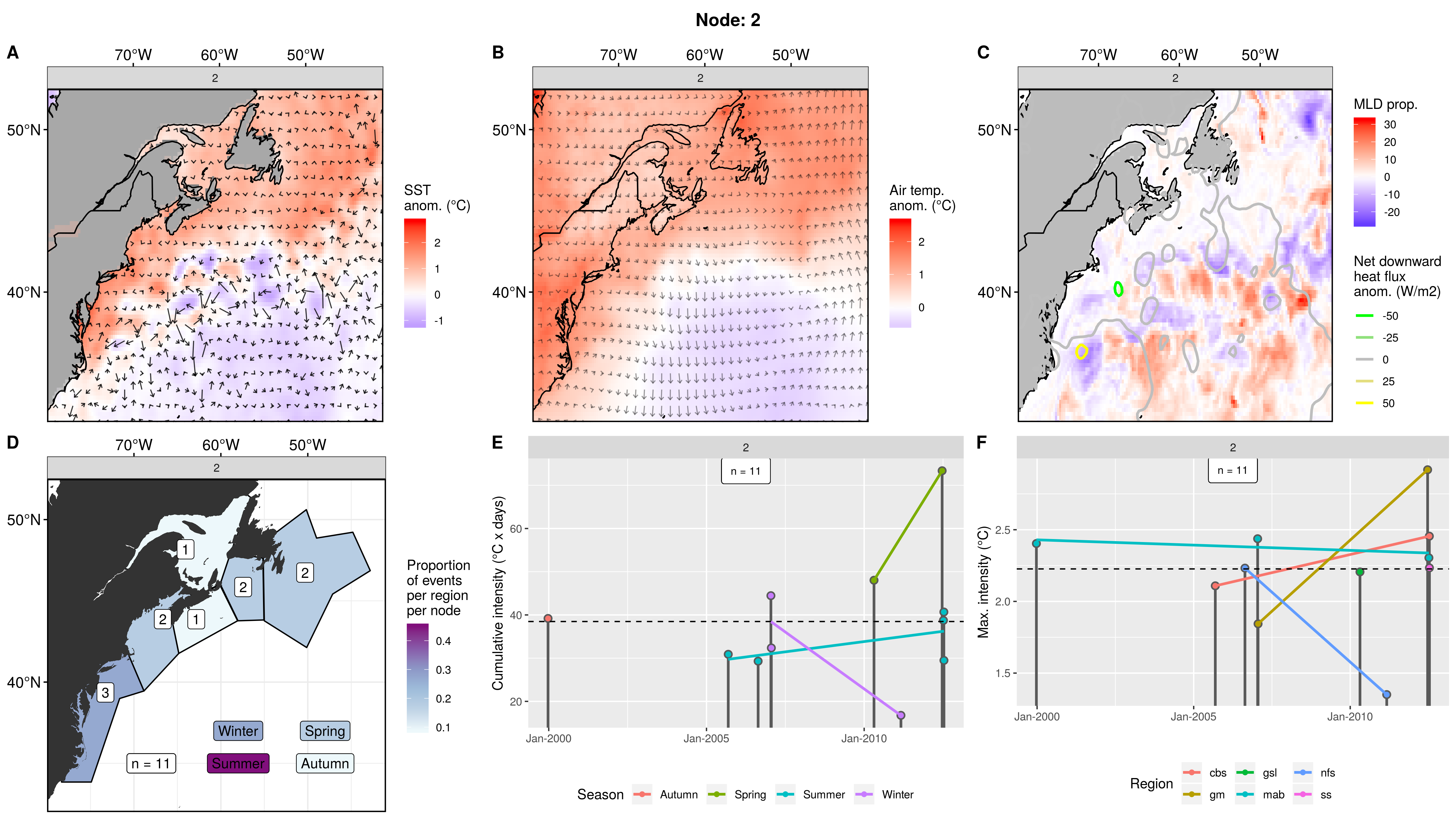
The table below contains a concise summary of the nodes following Table 4 in Oliver et al. (2018). The following sub-sections provide more in-depth explanations.
| Node | Region | Season | MHW Properties | Conditions |
|---|---|---|---|---|
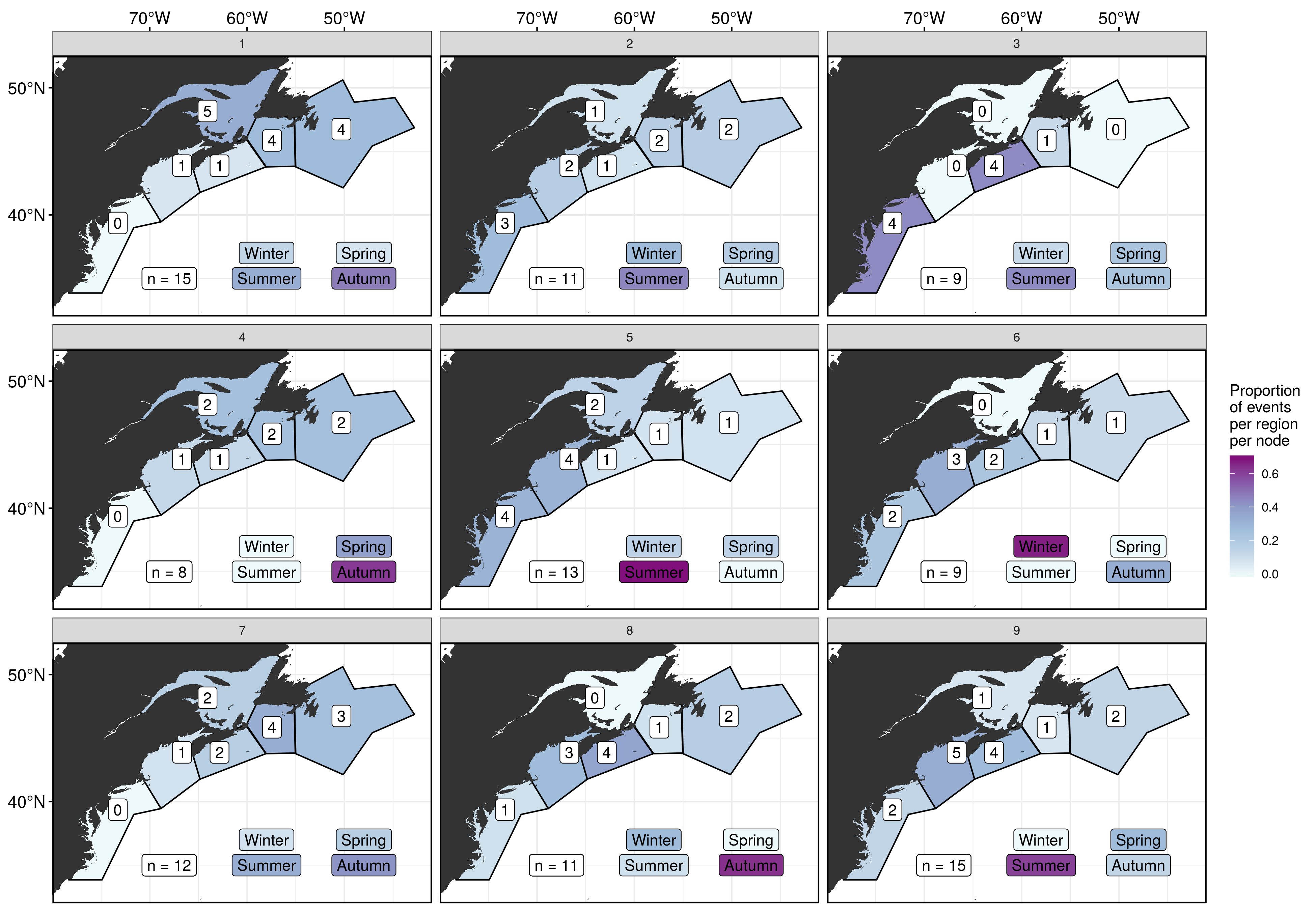
| 1 |
Season + region
Expand here to see past versions of fig_5.png:
| Version | Author | Date |
|---|---|---|
| 9273f18 | robwschlegel | 2019-08-11 |
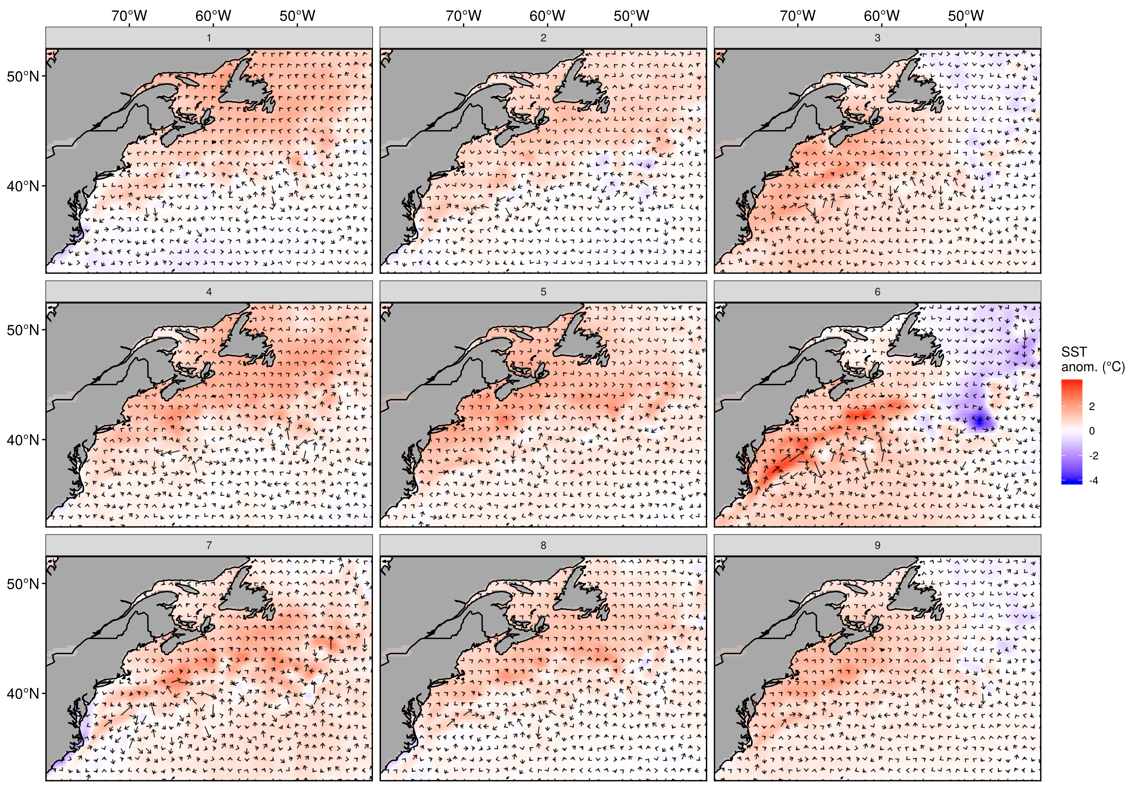
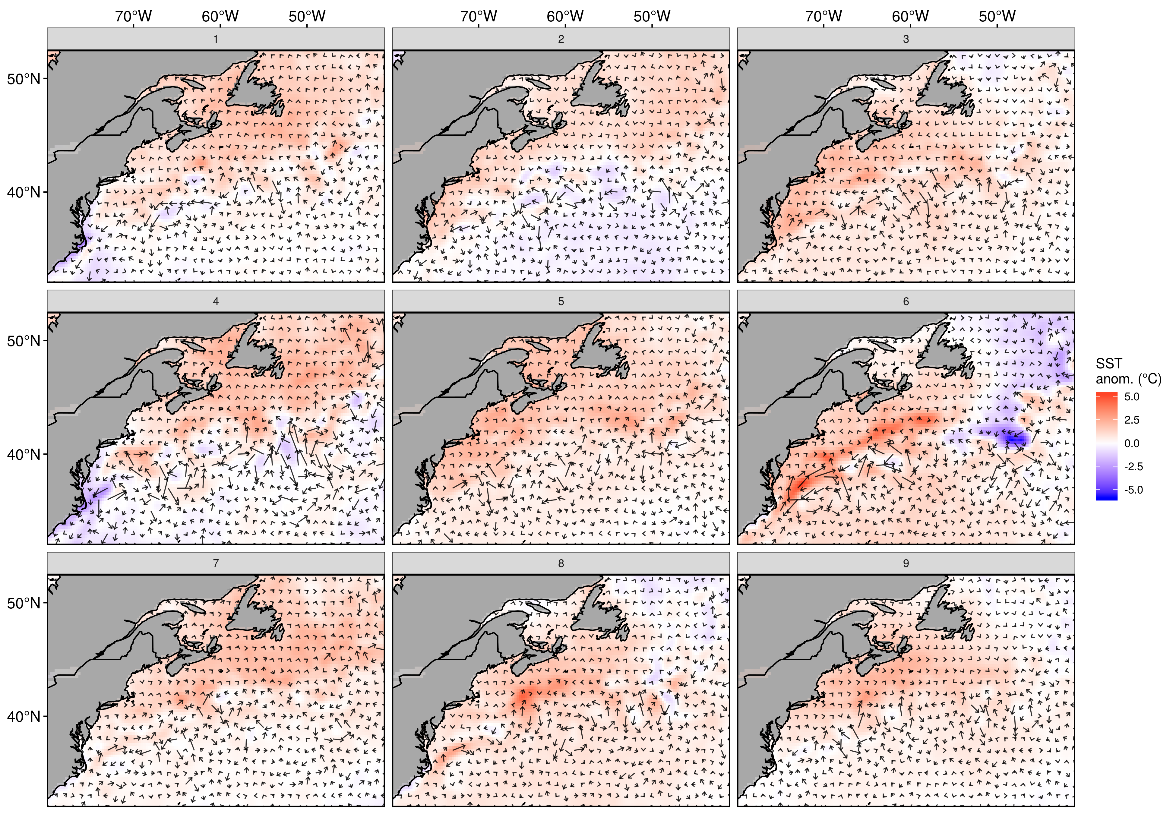
SST + U + V
Expand here to see past versions of fig_2.png:
| Version | Author | Date |
|---|---|---|
| 9273f18 | robwschlegel | 2019-08-11 |
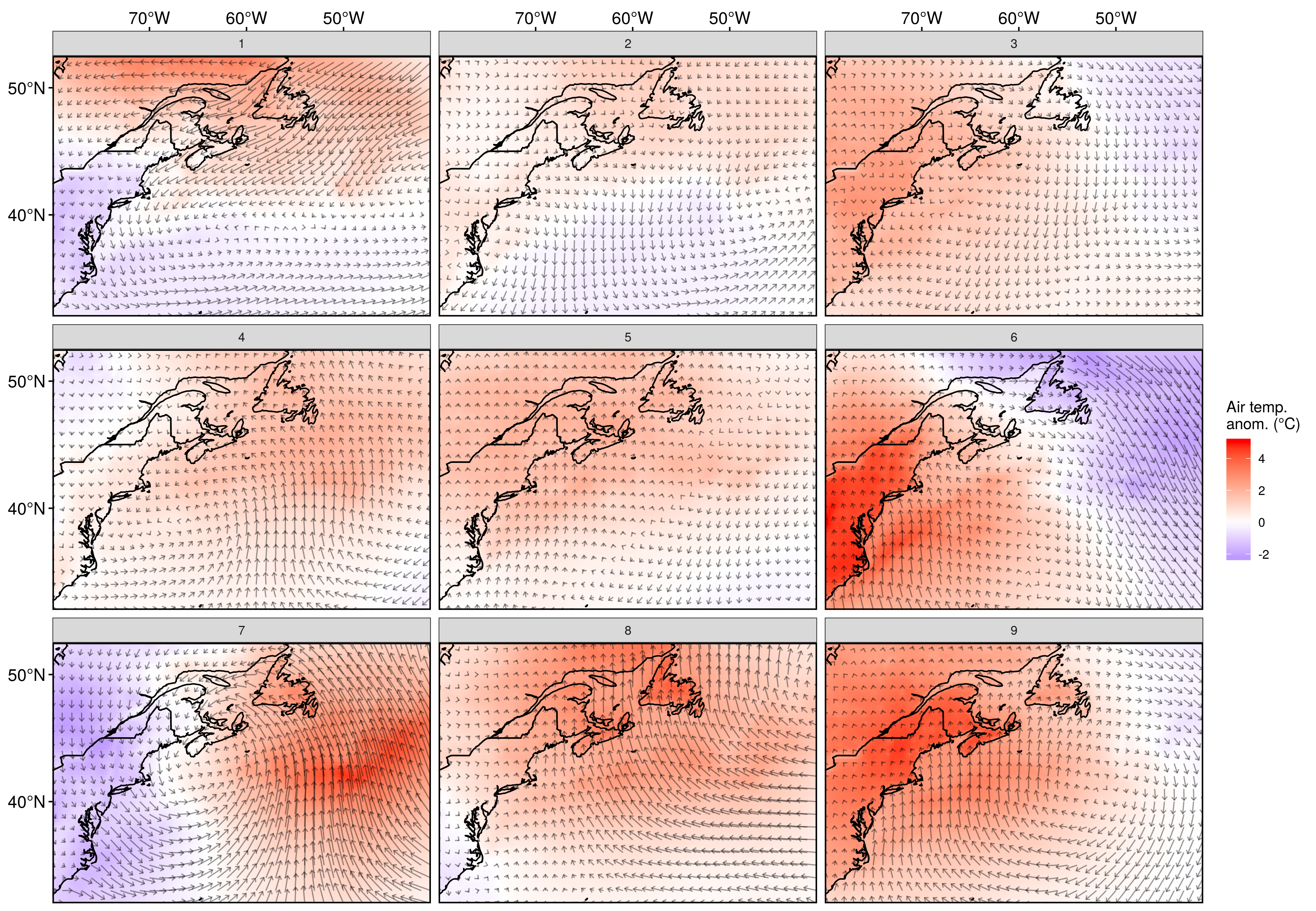
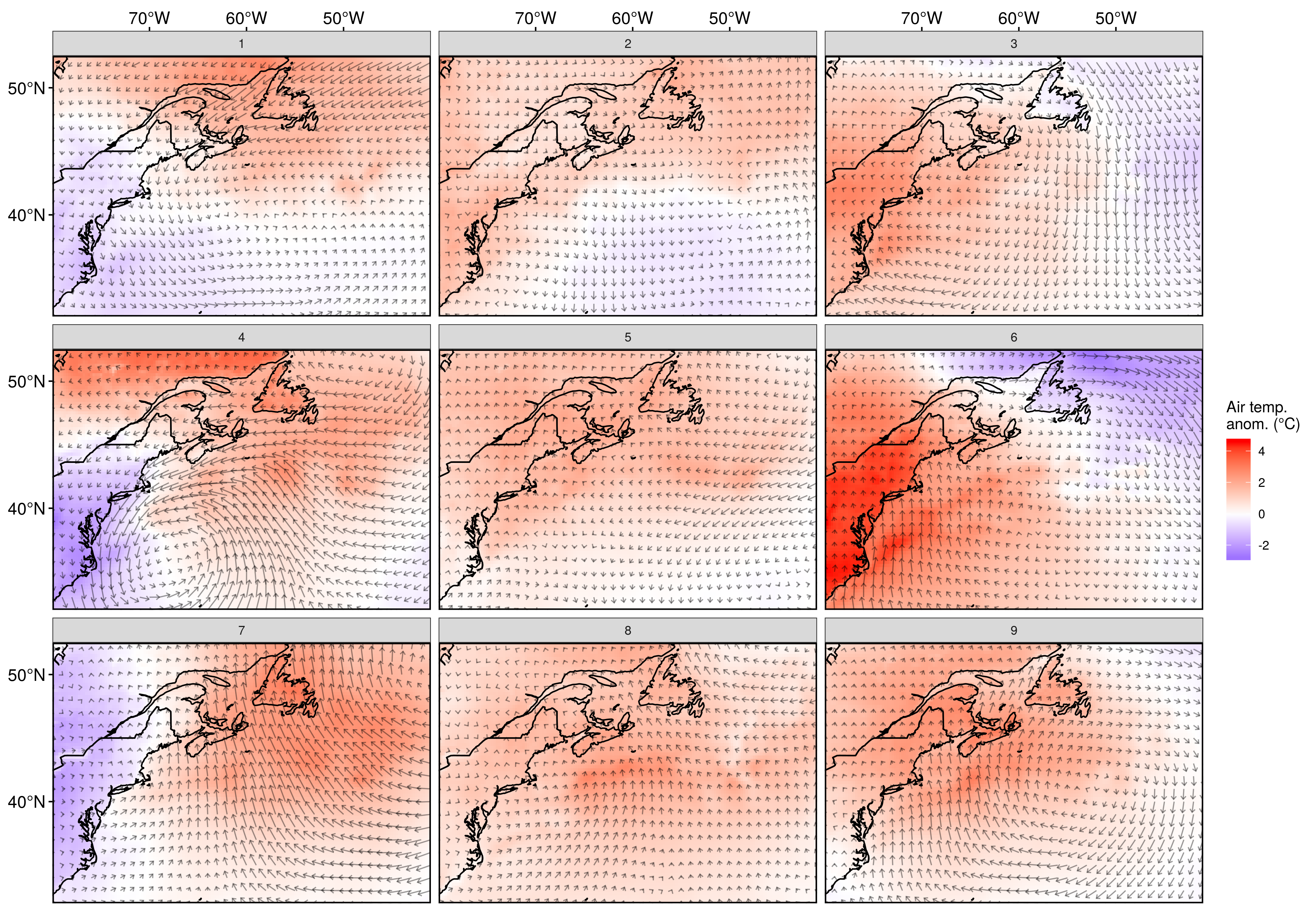
Air temp + U + V
Expand here to see past versions of fig_3.png:
| Version | Author | Date |
|---|---|---|
| 9273f18 | robwschlegel | 2019-08-11 |
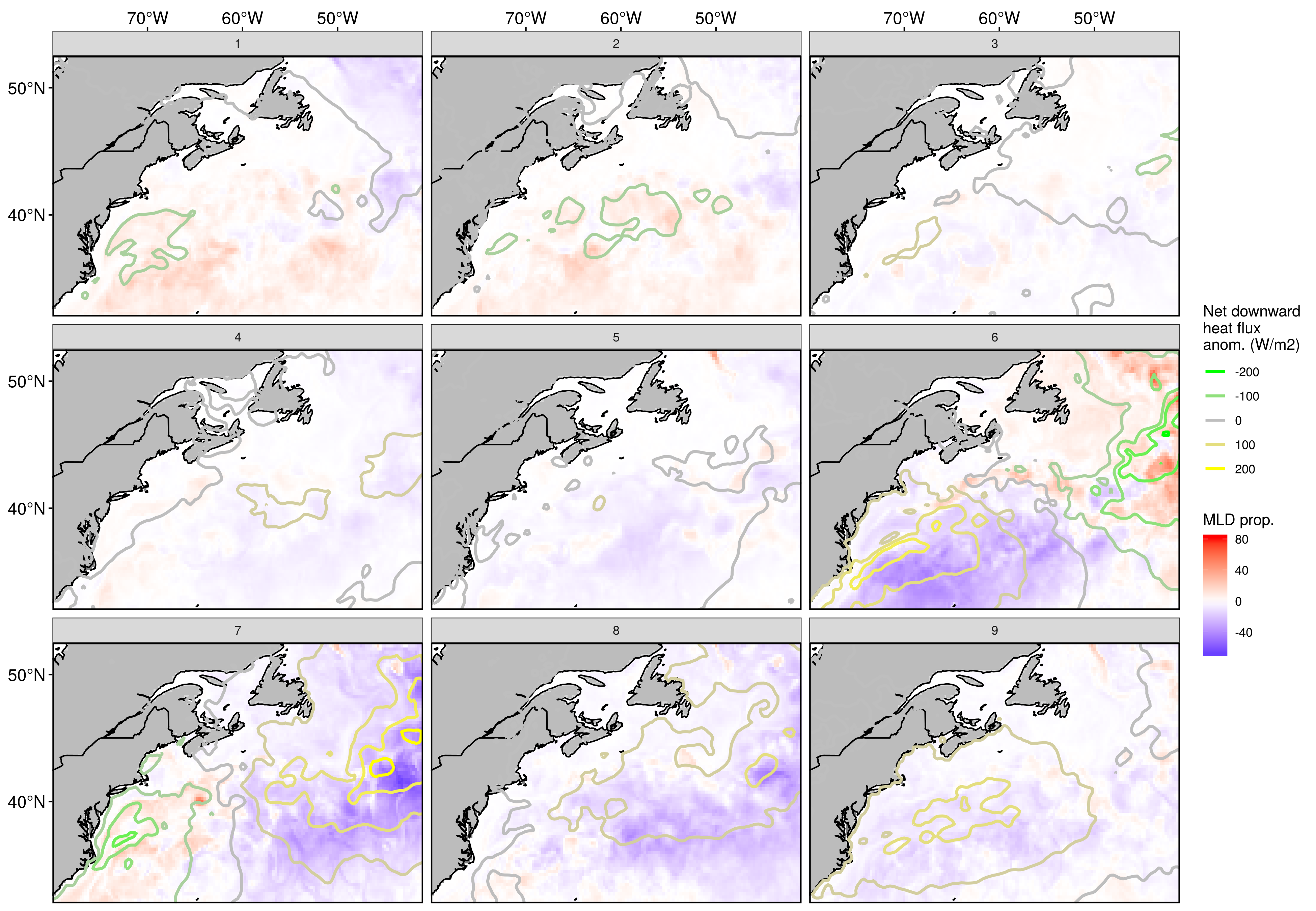
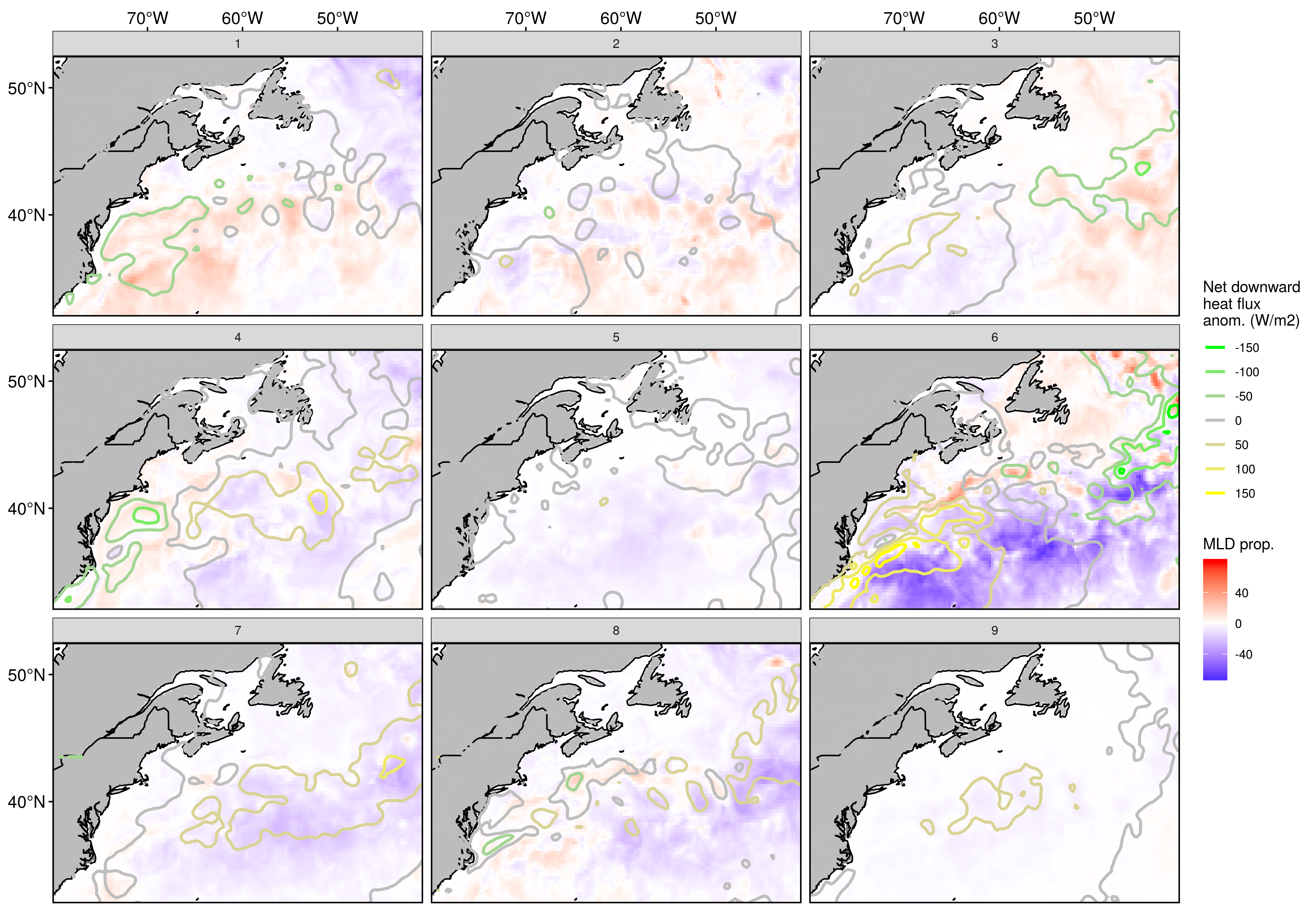
MLD + Net downward heatflux
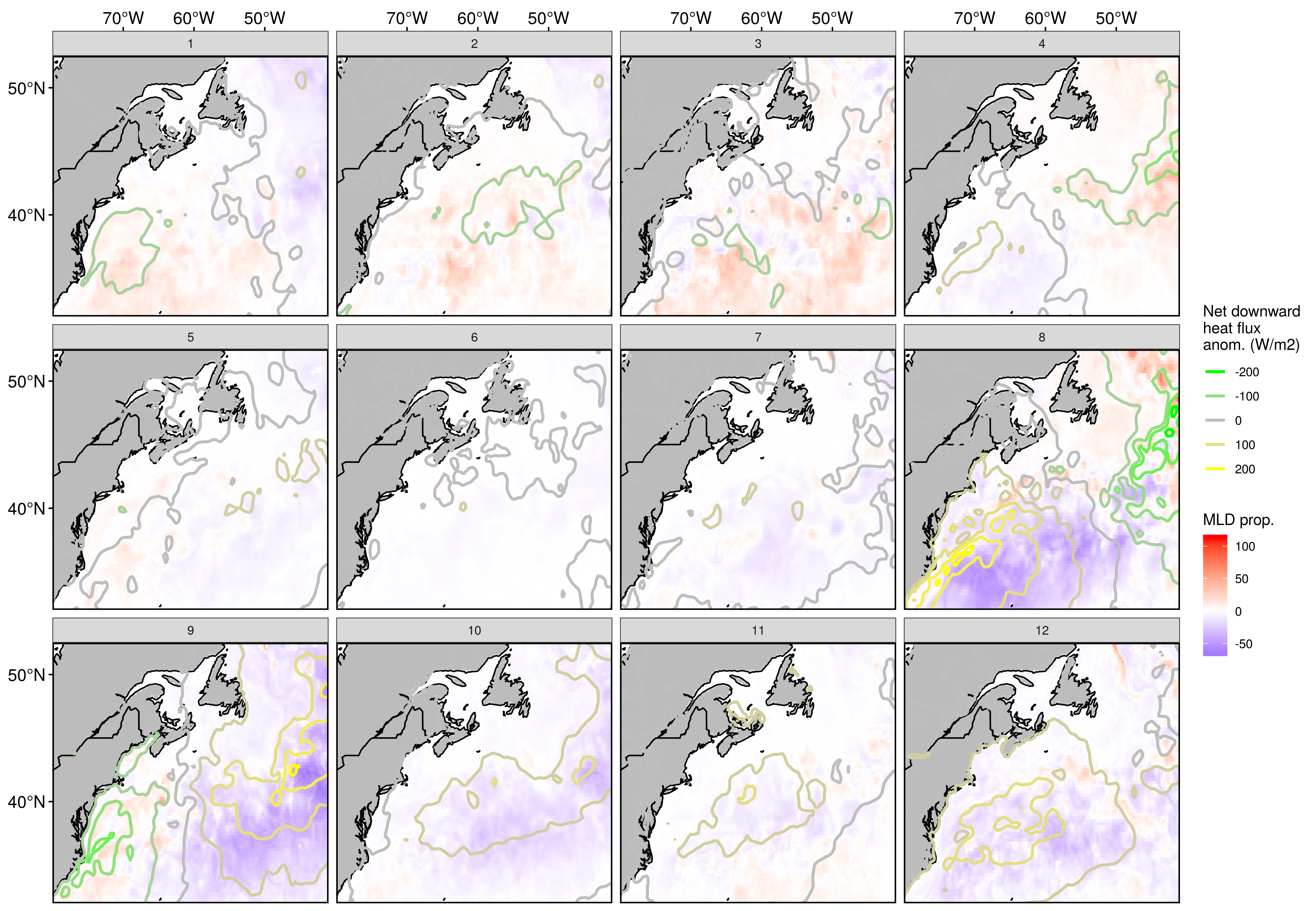
Expand here to see past versions of fig_4.png:
| Version | Author | Date |
|---|---|---|
| 9273f18 | robwschlegel | 2019-08-11 |
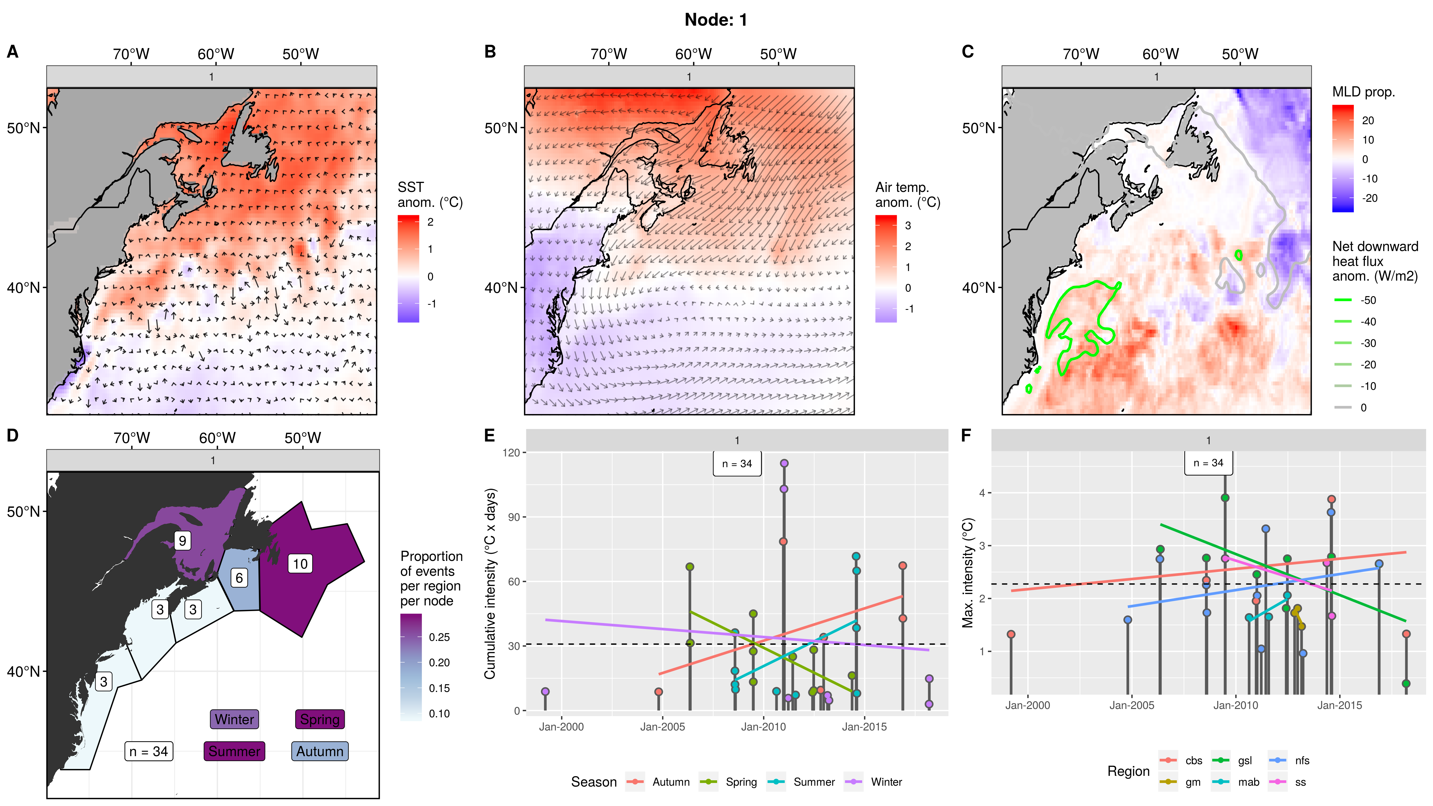
Node 1
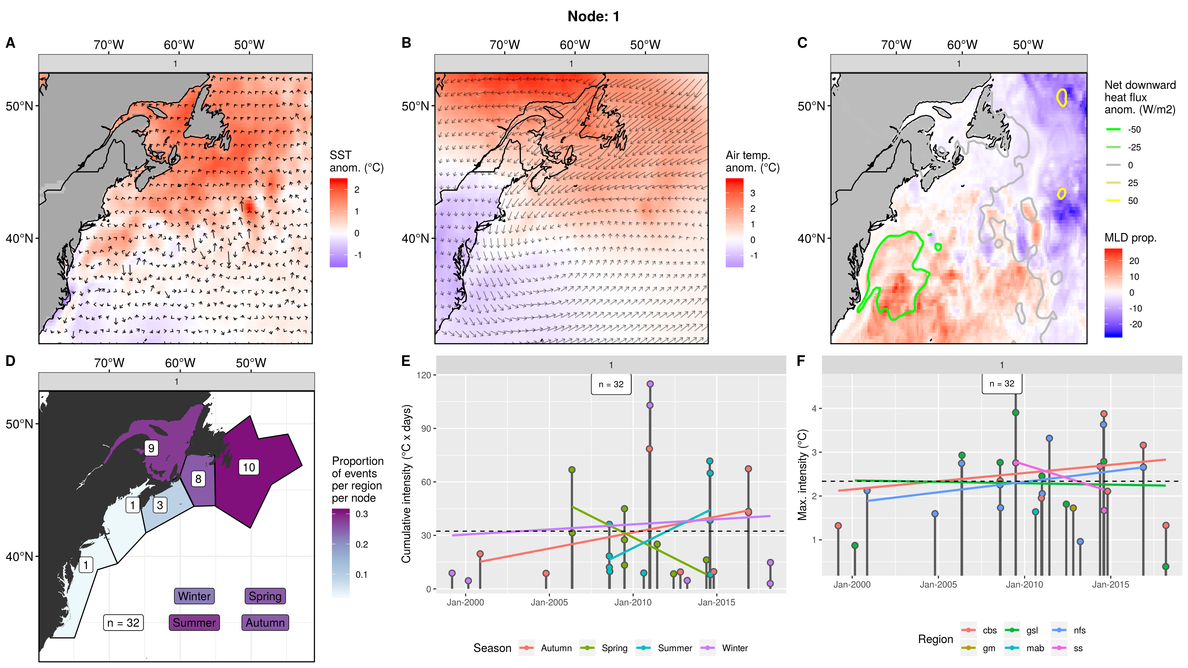
Expand here to see past versions of node_1_panels.png:
| Version | Author | Date |
|---|---|---|
| 9273f18 | robwschlegel | 2019-08-11 |
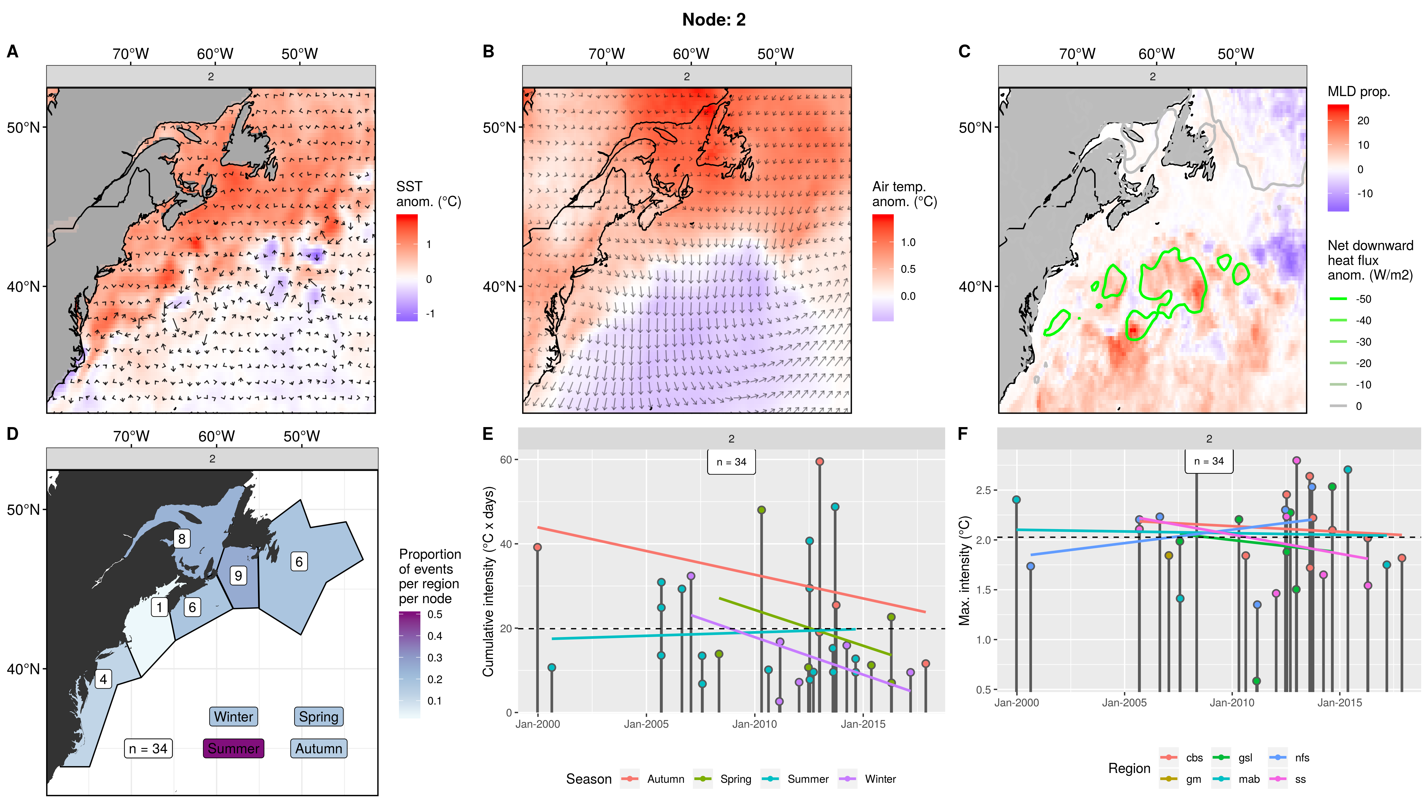
Node 2
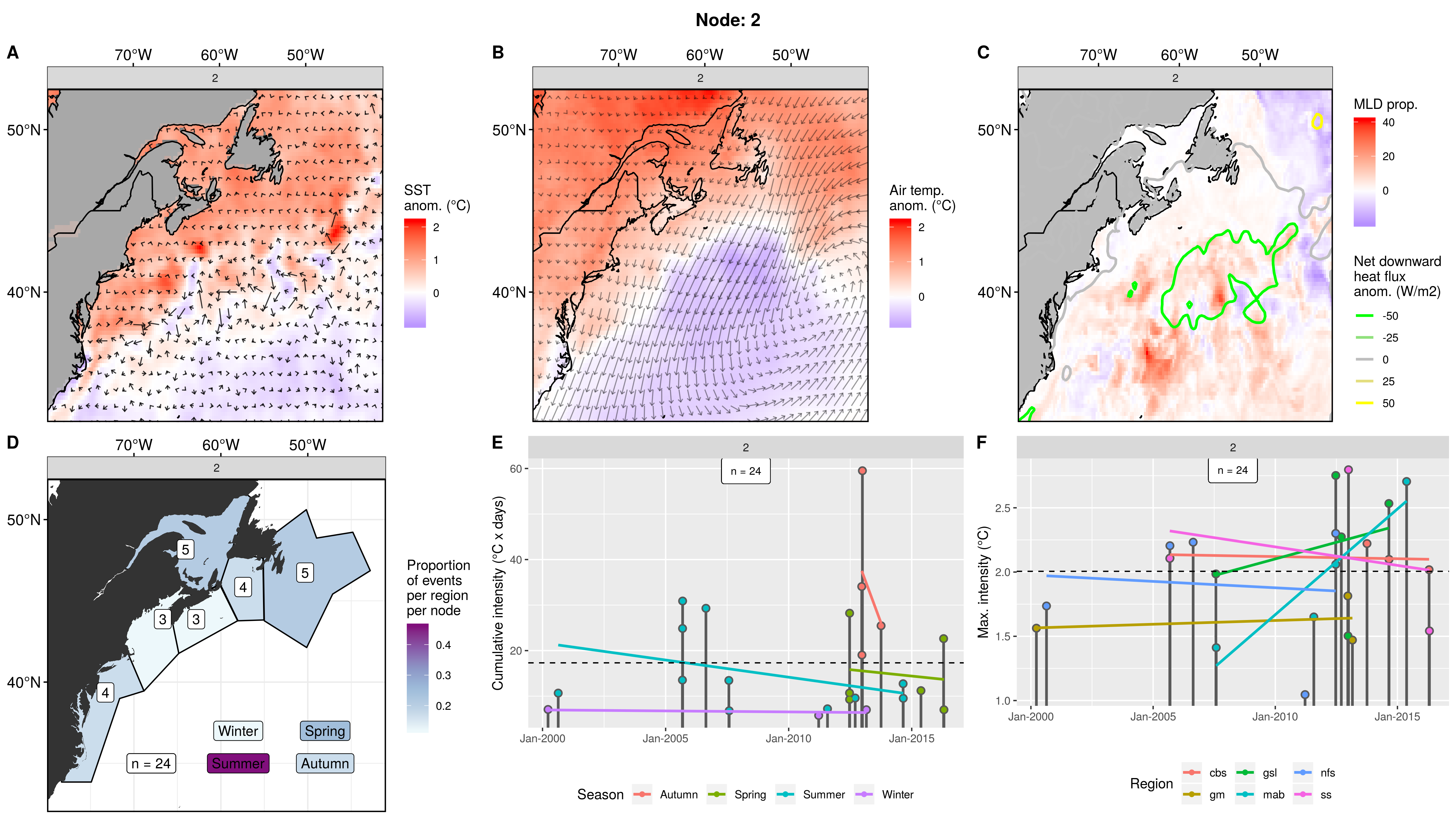
Expand here to see past versions of node_2_panels.png:
| Version | Author | Date |
|---|---|---|
| 9273f18 | robwschlegel | 2019-08-11 |
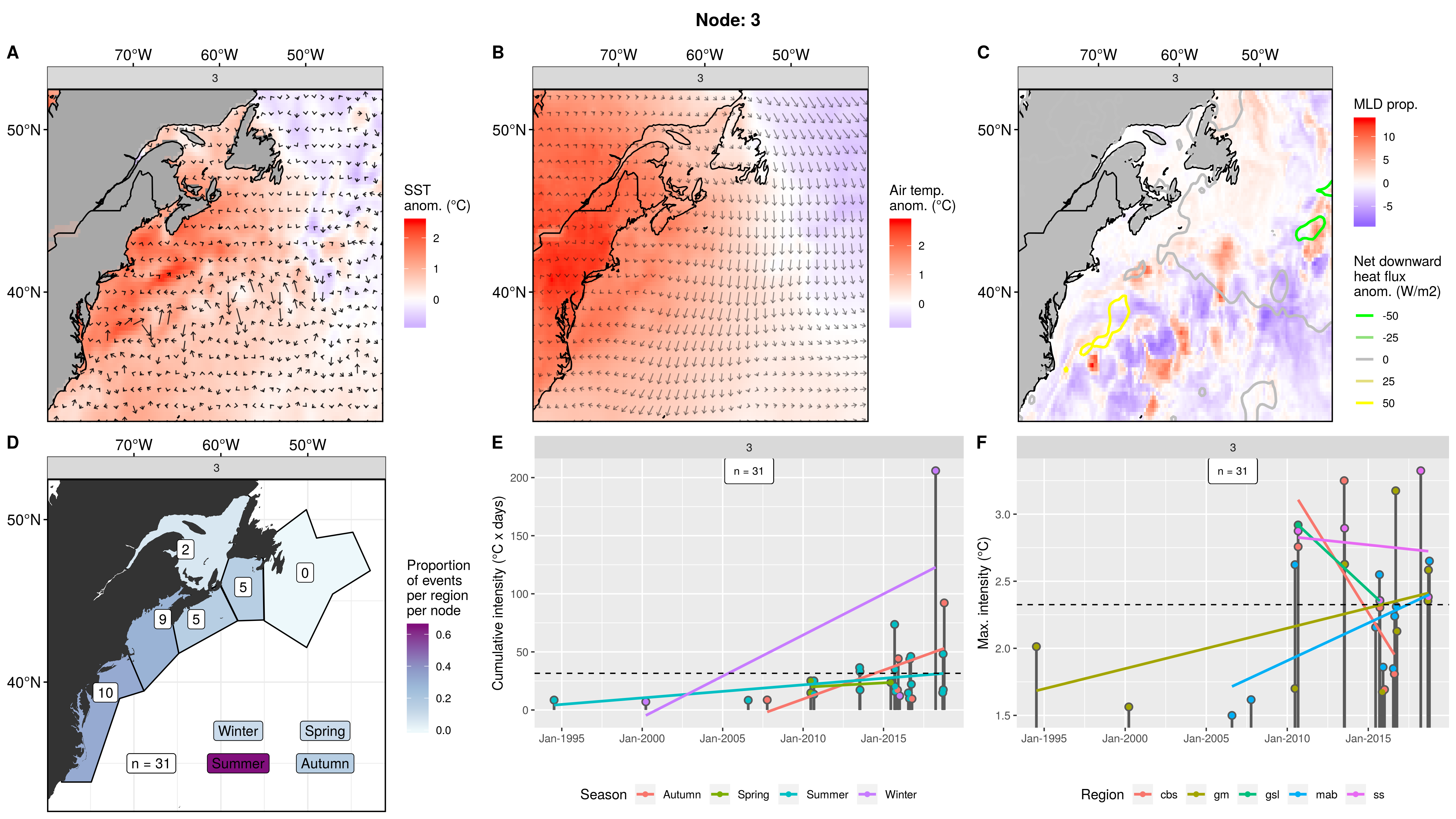
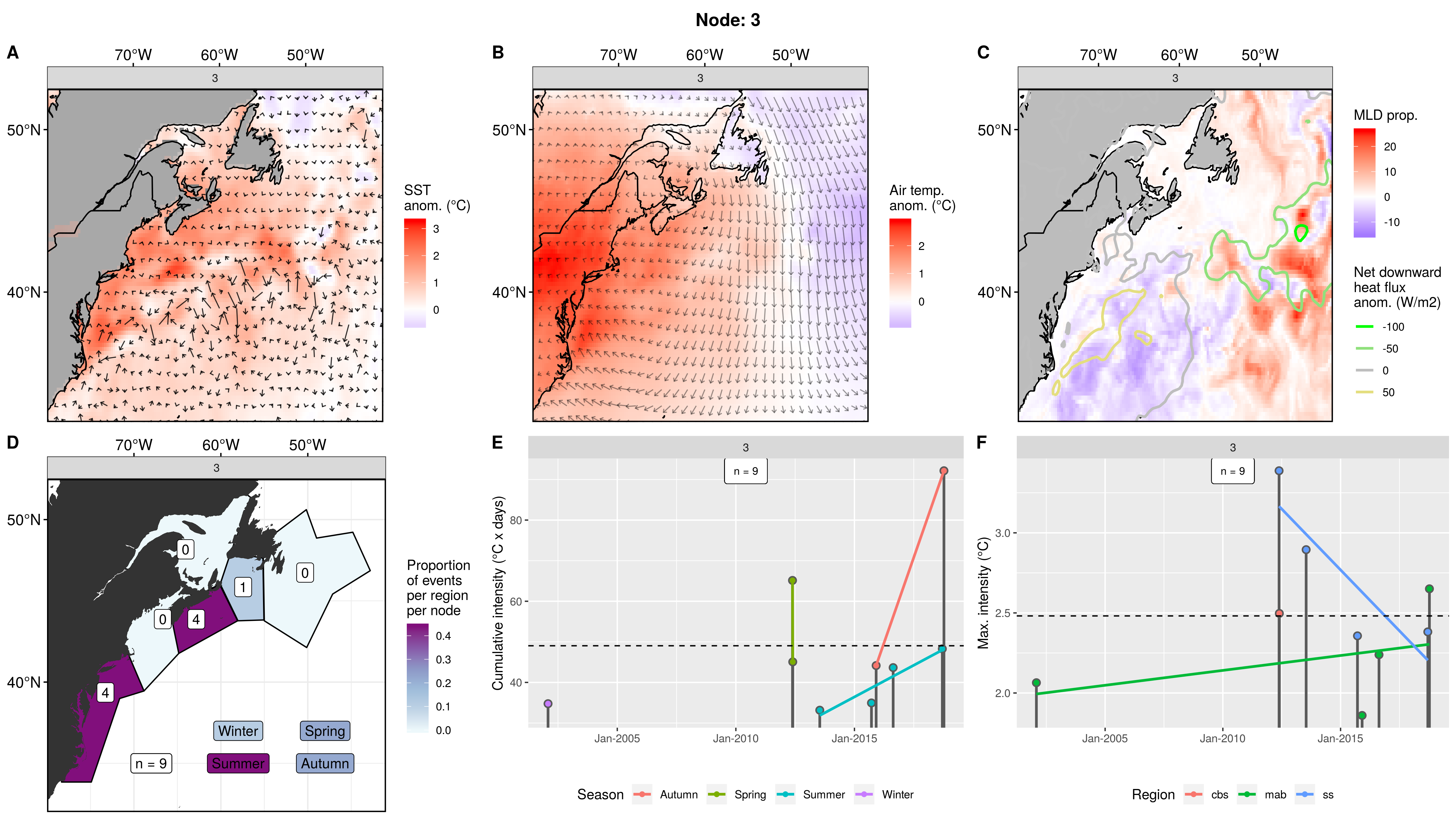
Node 3
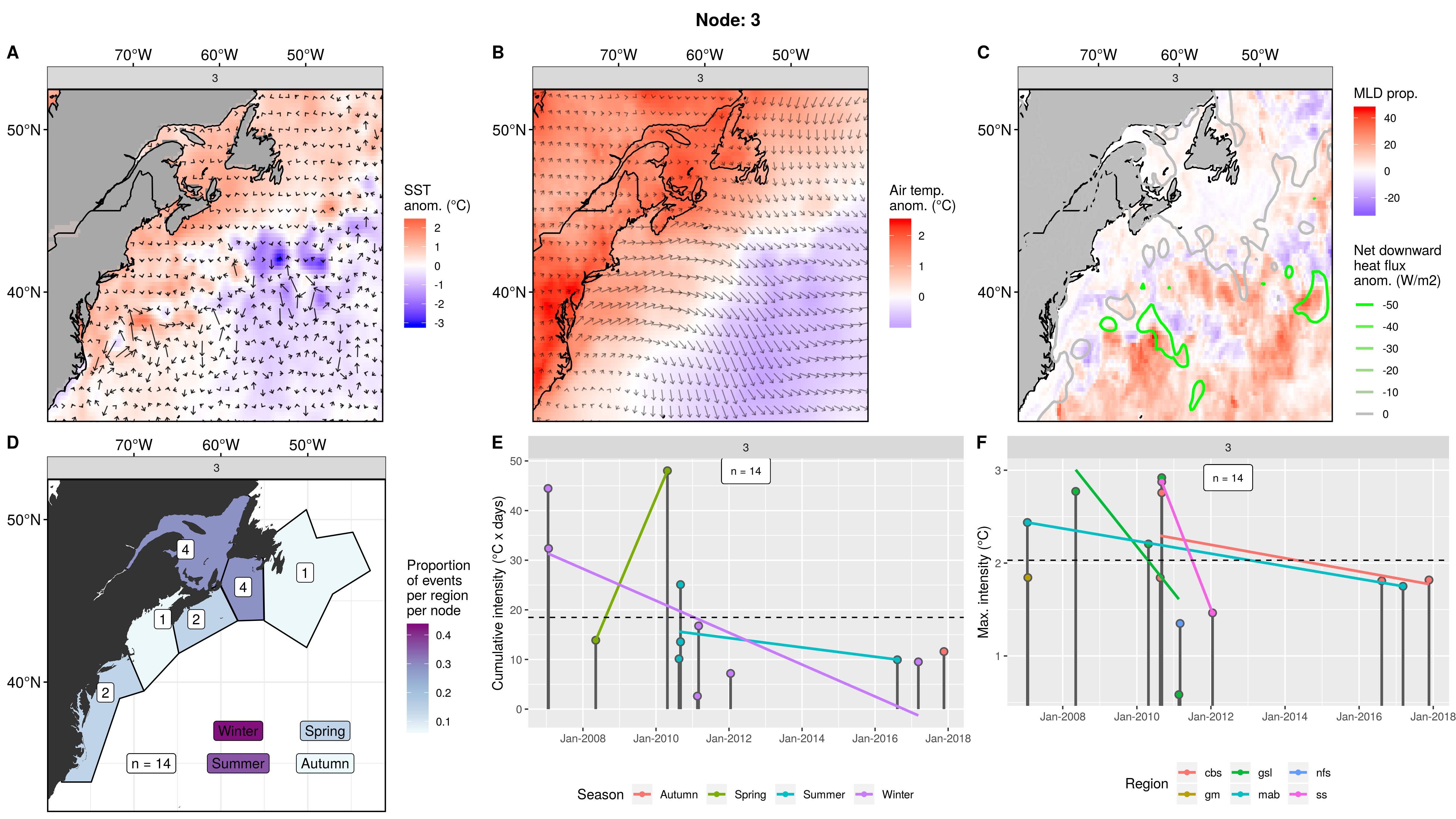
Expand here to see past versions of node_3_panels.png:
| Version | Author | Date |
|---|---|---|
| 9273f18 | robwschlegel | 2019-08-11 |
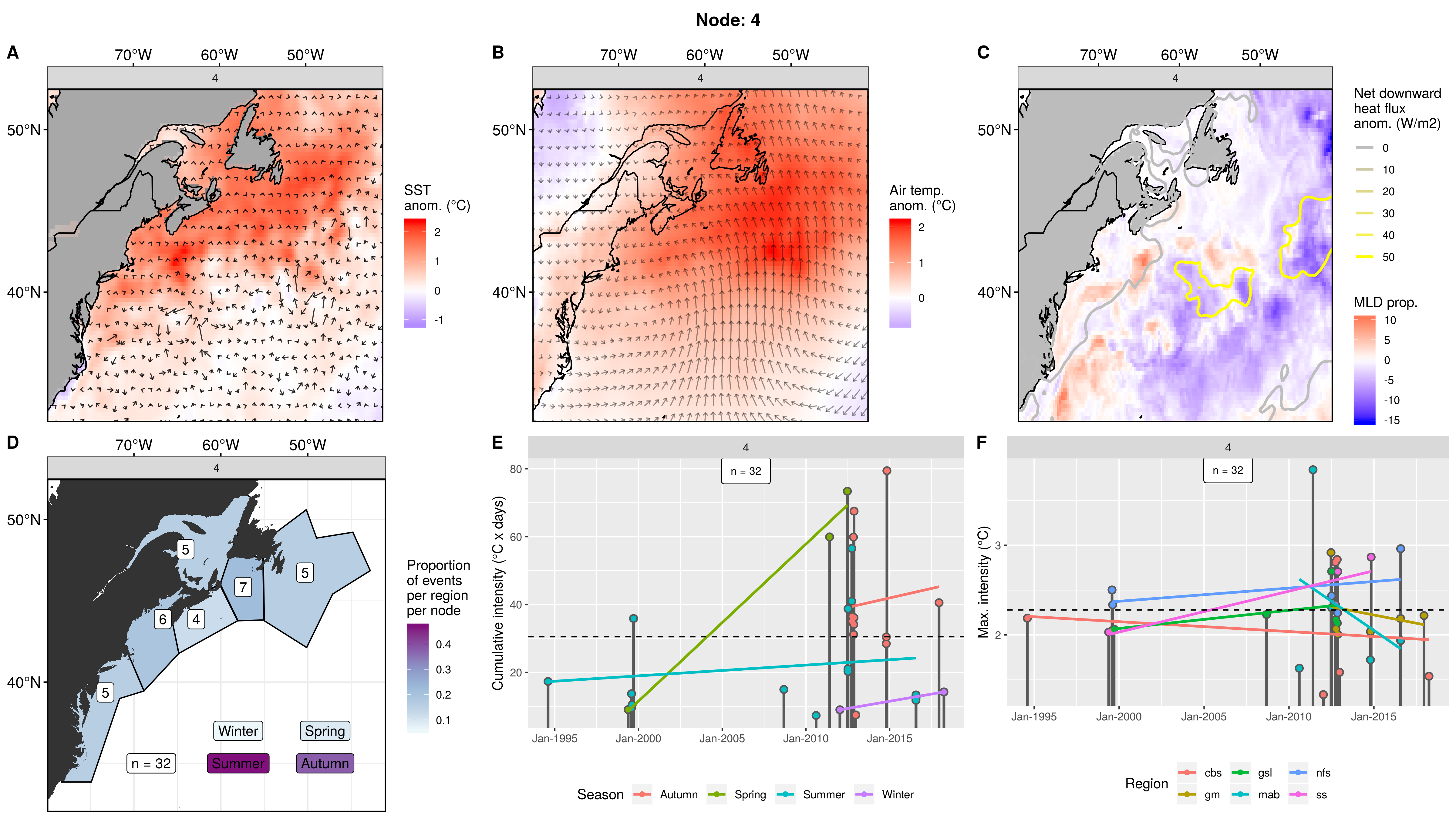
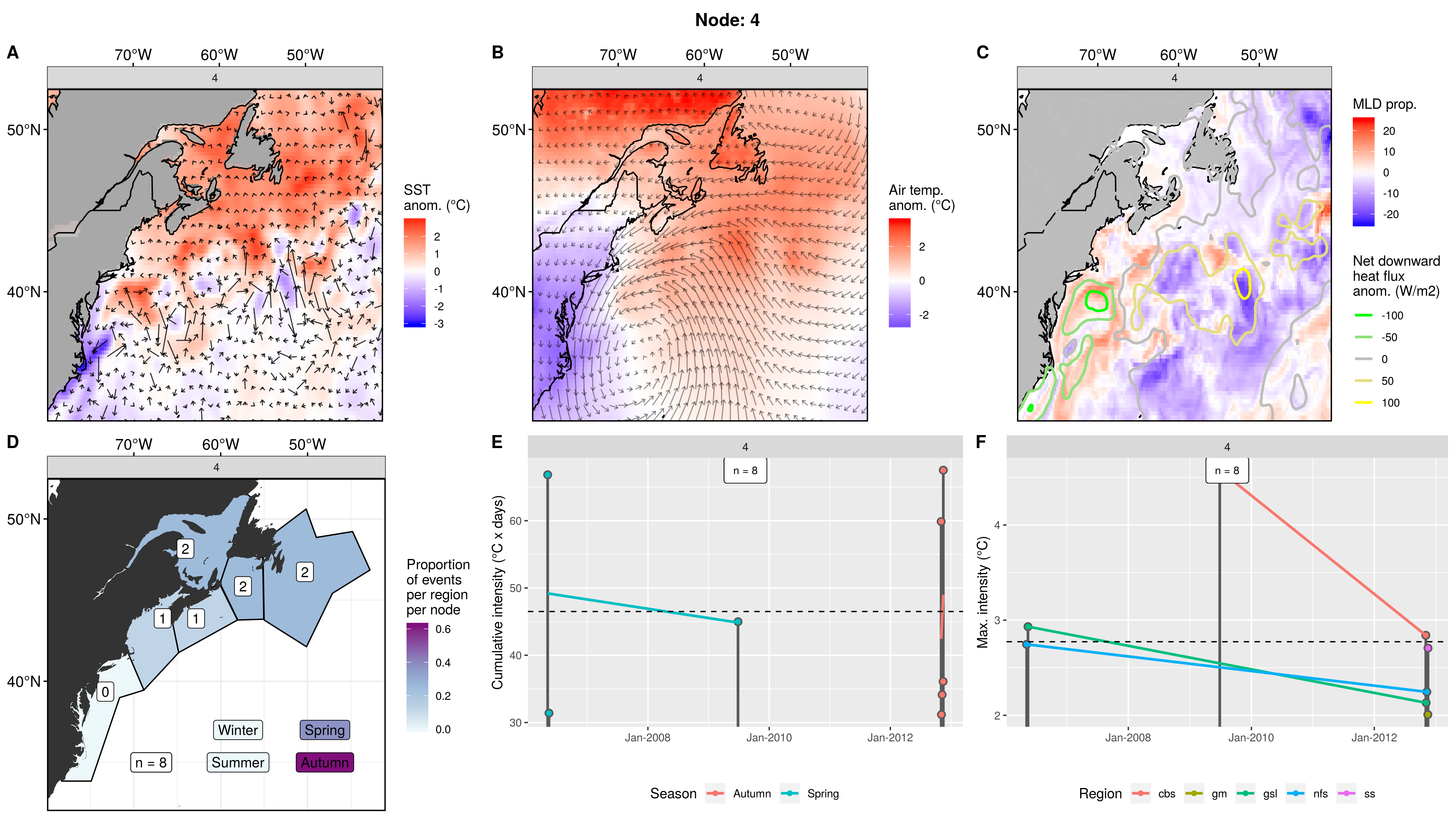
Node 4
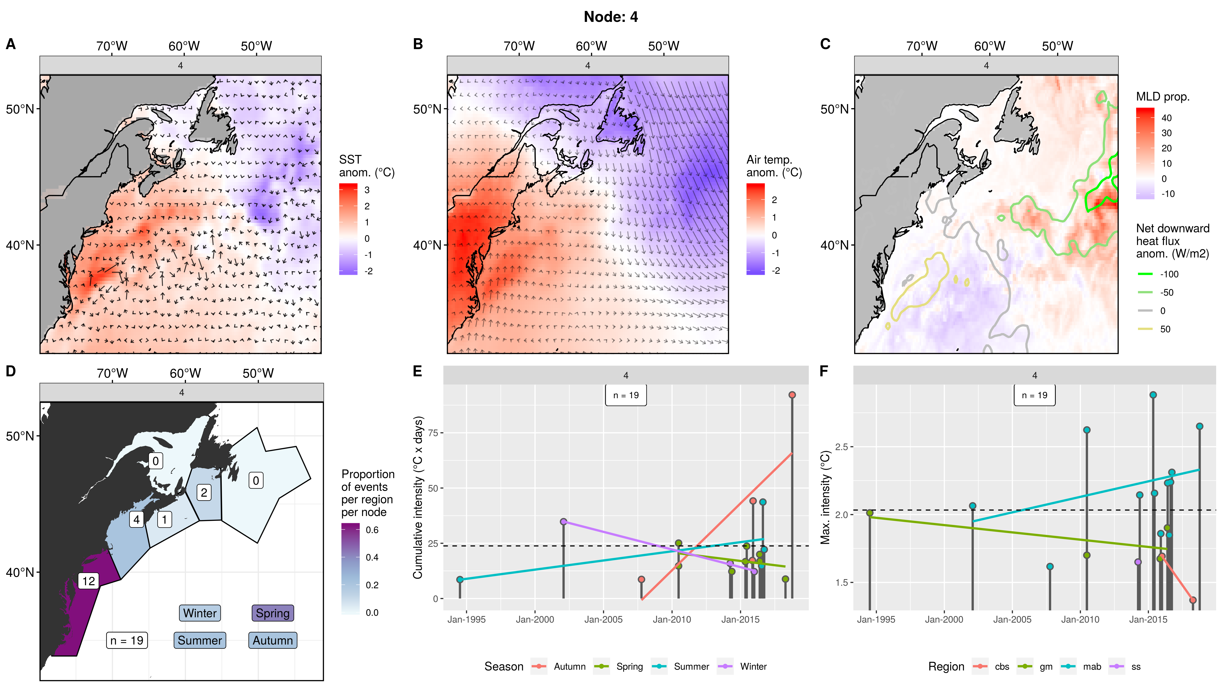
Expand here to see past versions of node_4_panels.png:
| Version | Author | Date |
|---|---|---|
| 9273f18 | robwschlegel | 2019-08-11 |
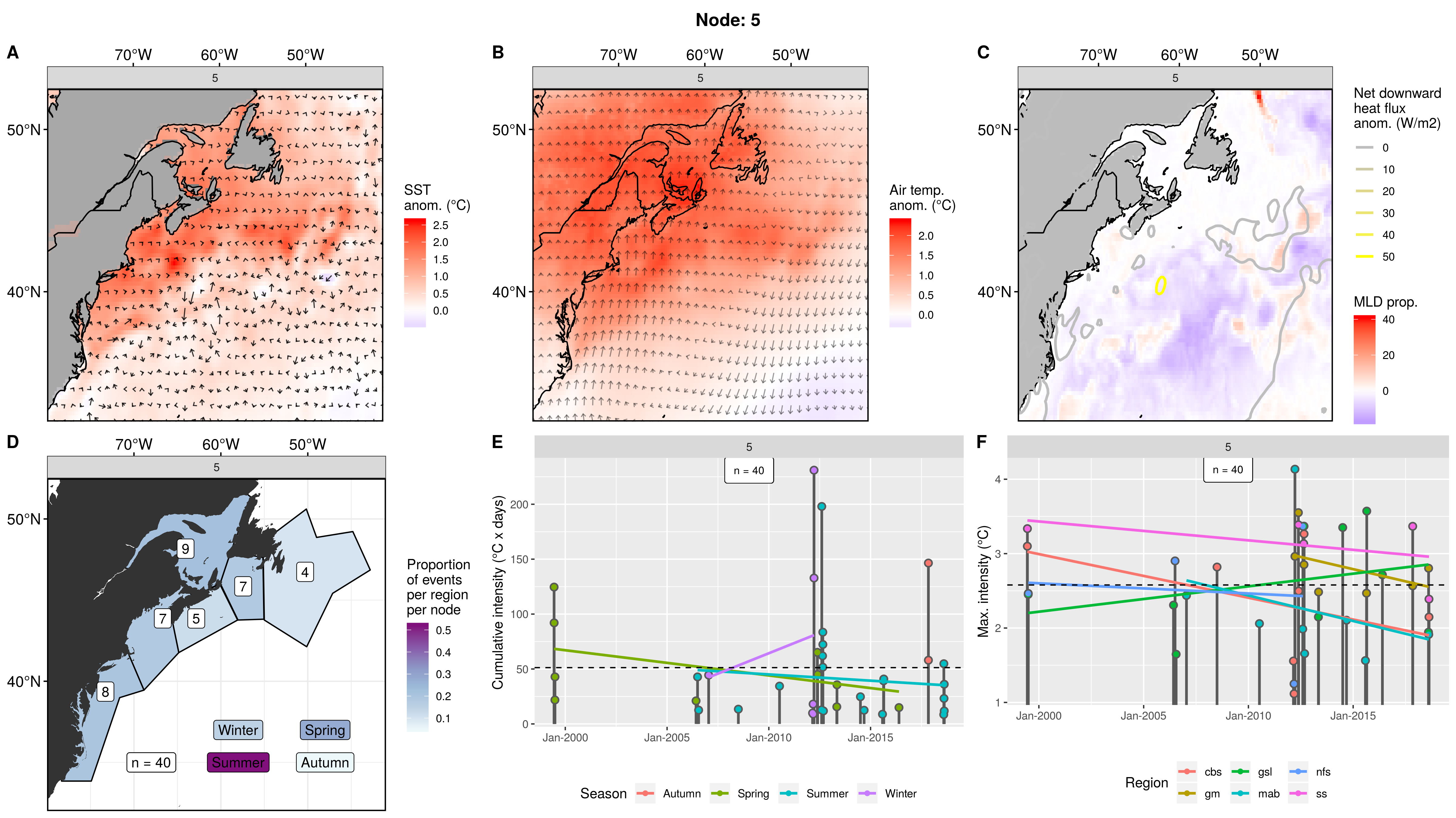
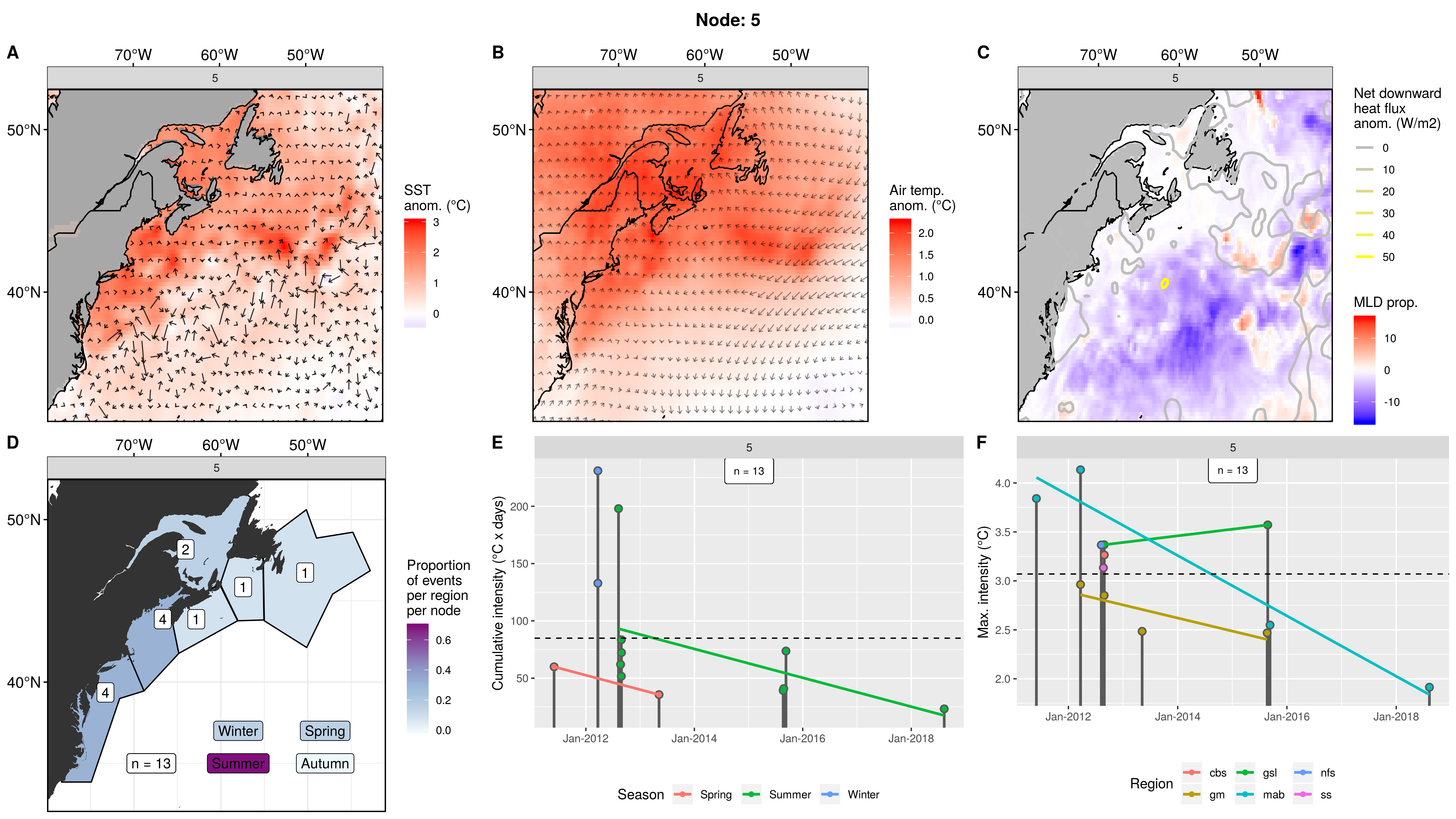
Node 5
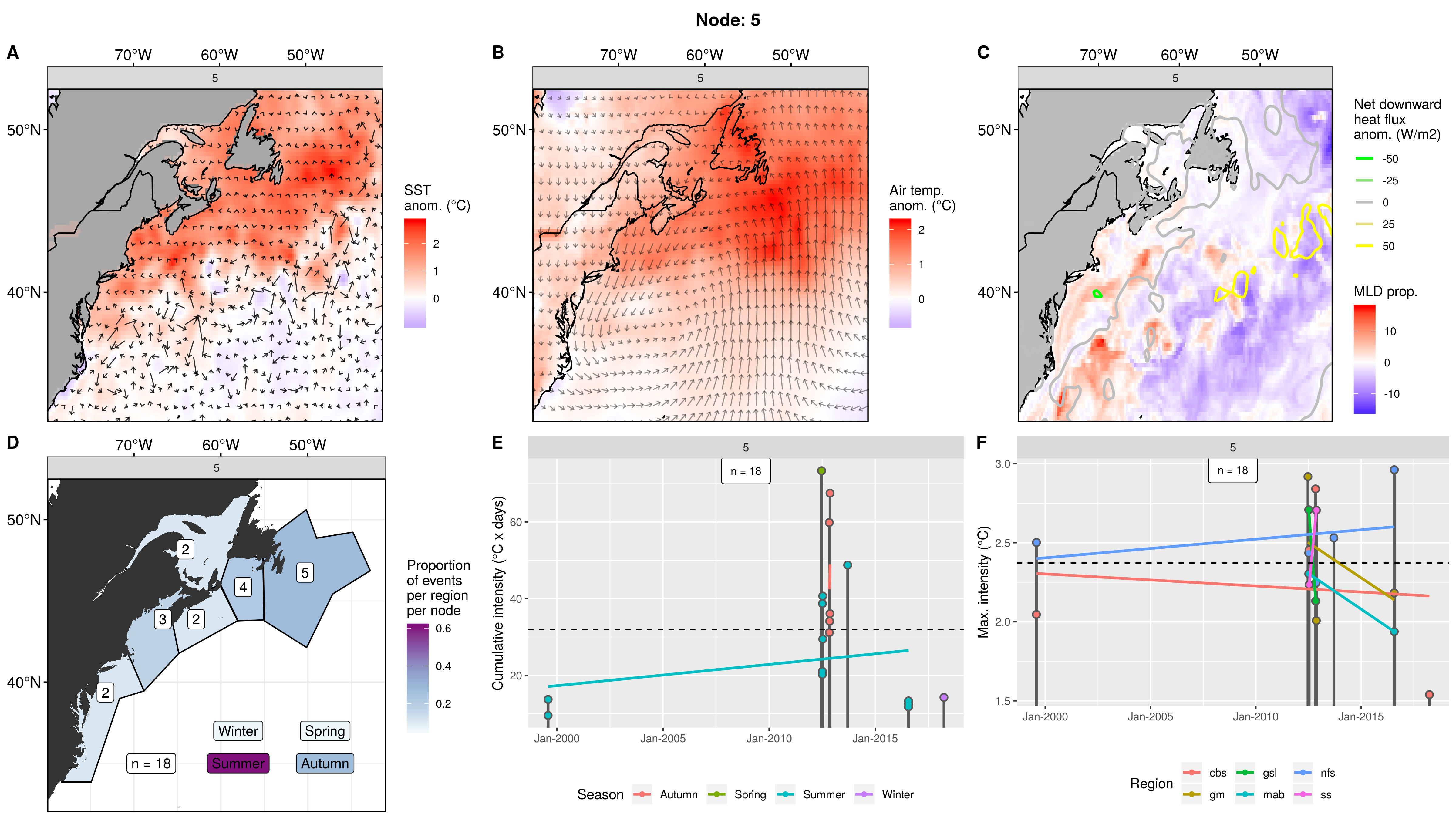
Expand here to see past versions of node_5_panels.png:
| Version | Author | Date |
|---|---|---|
| 9273f18 | robwschlegel | 2019-08-11 |
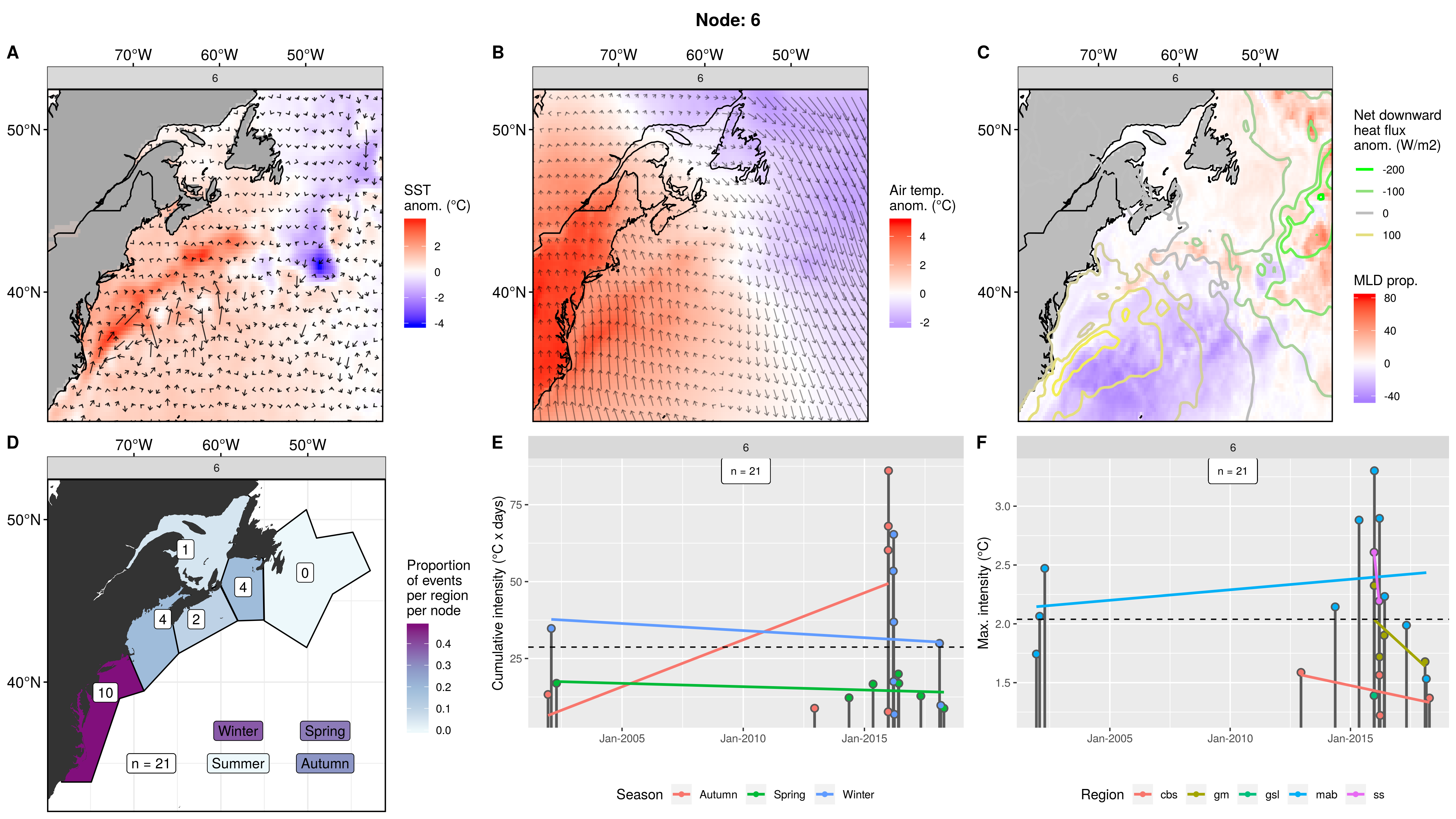
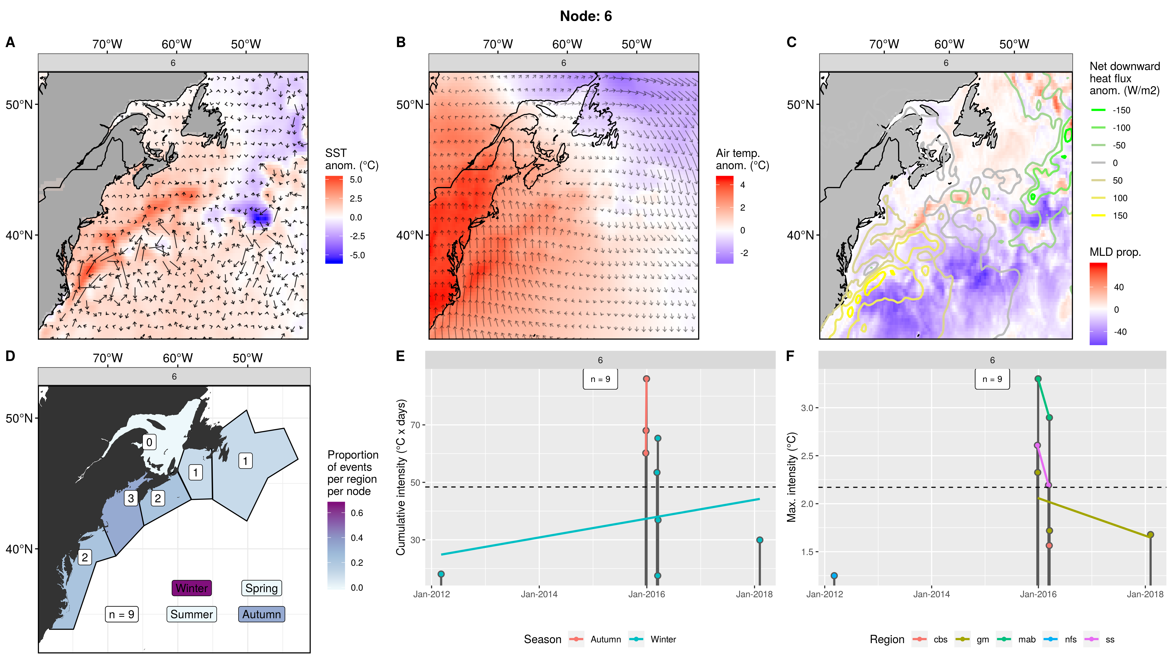
Node 6
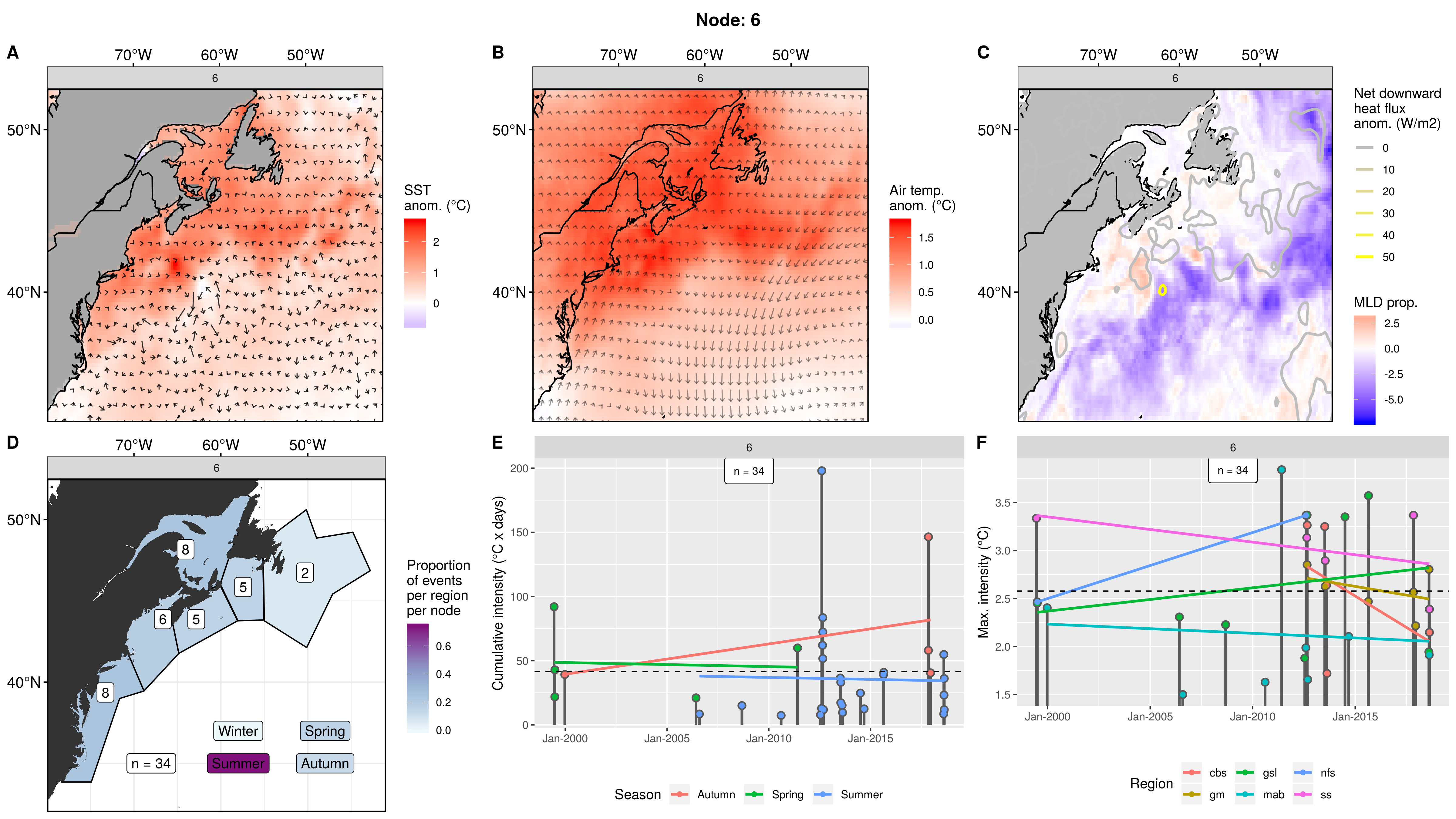
Expand here to see past versions of node_6_panels.png:
| Version | Author | Date |
|---|---|---|
| 9273f18 | robwschlegel | 2019-08-11 |
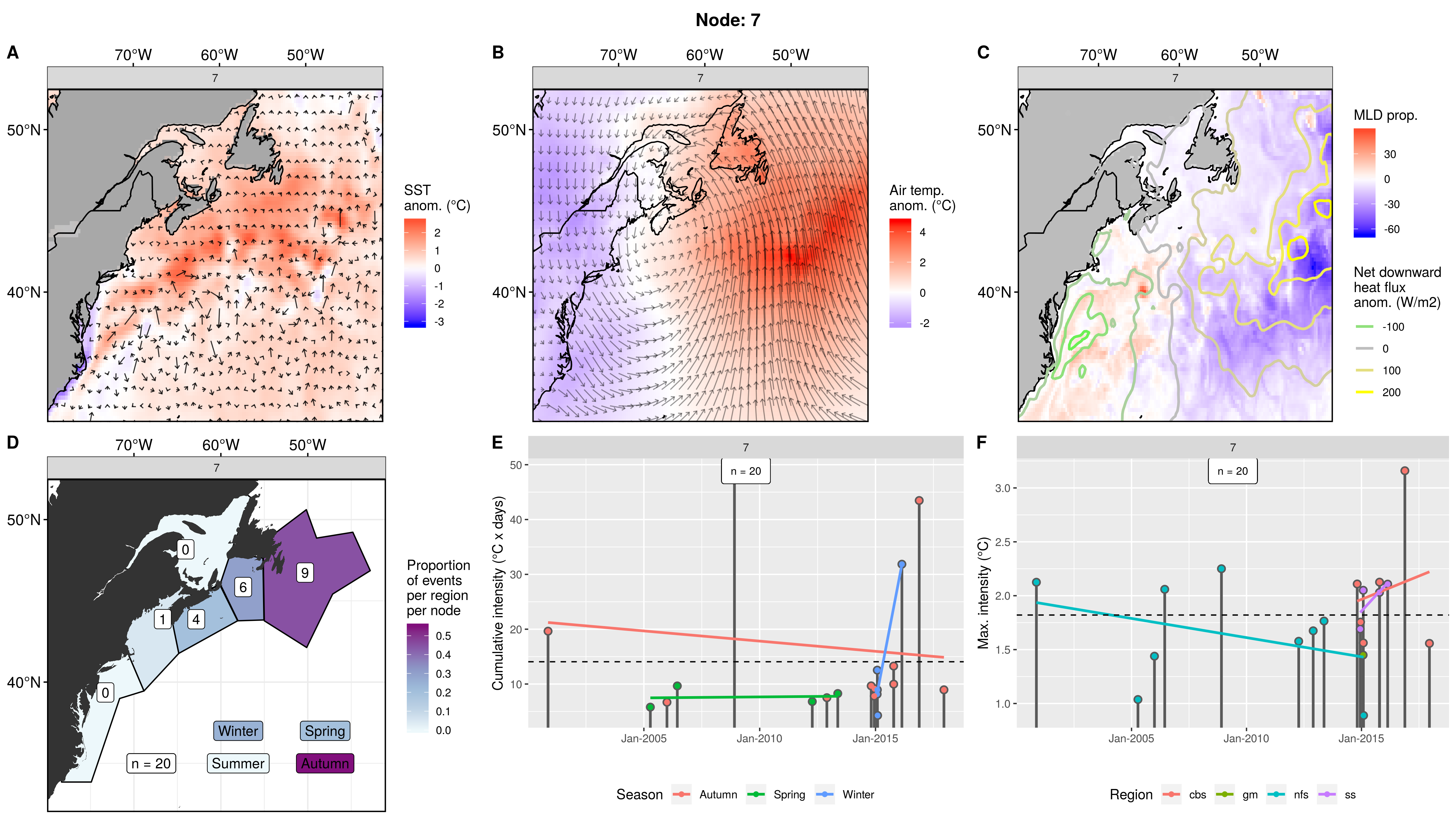
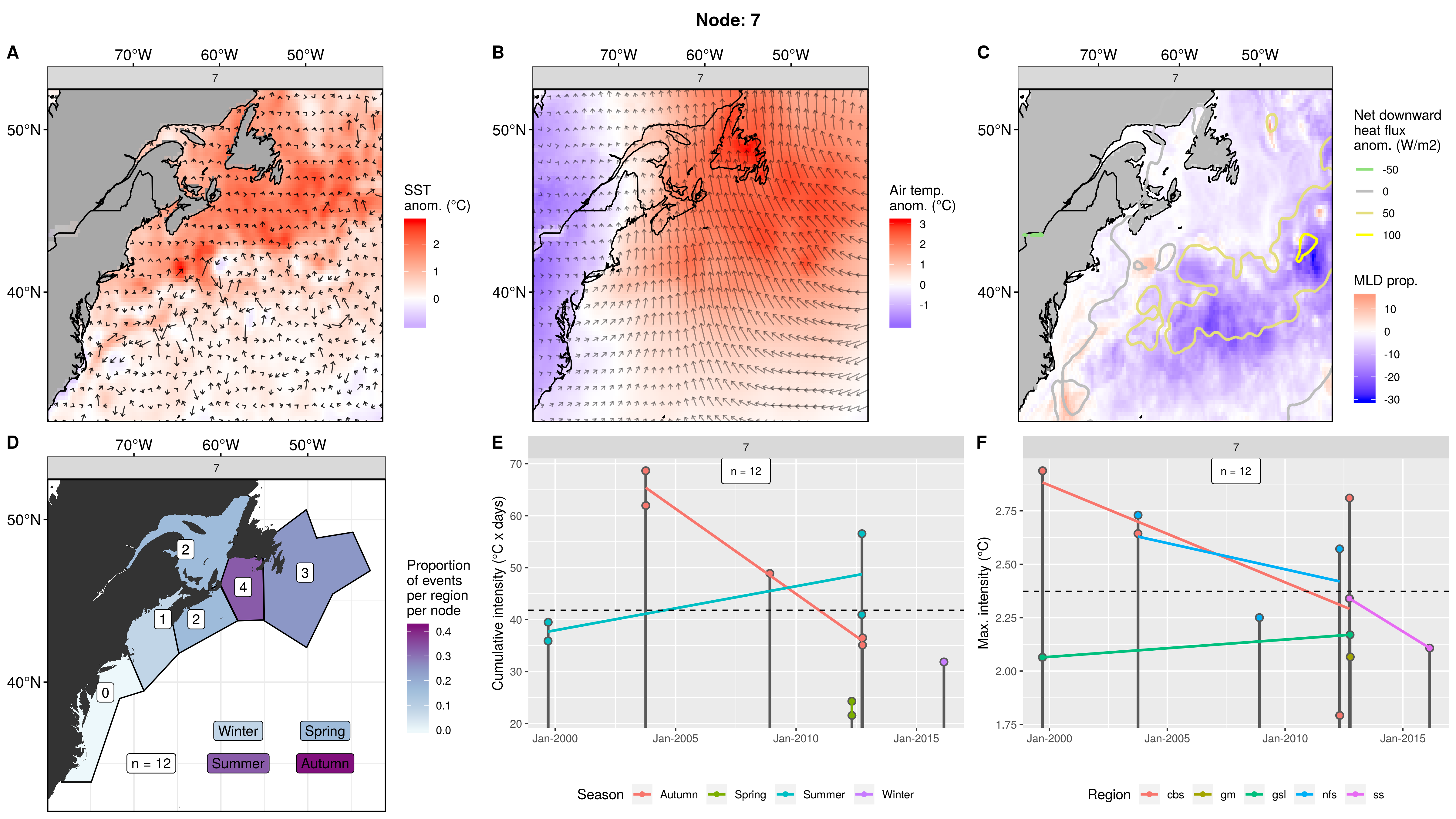
Node 7
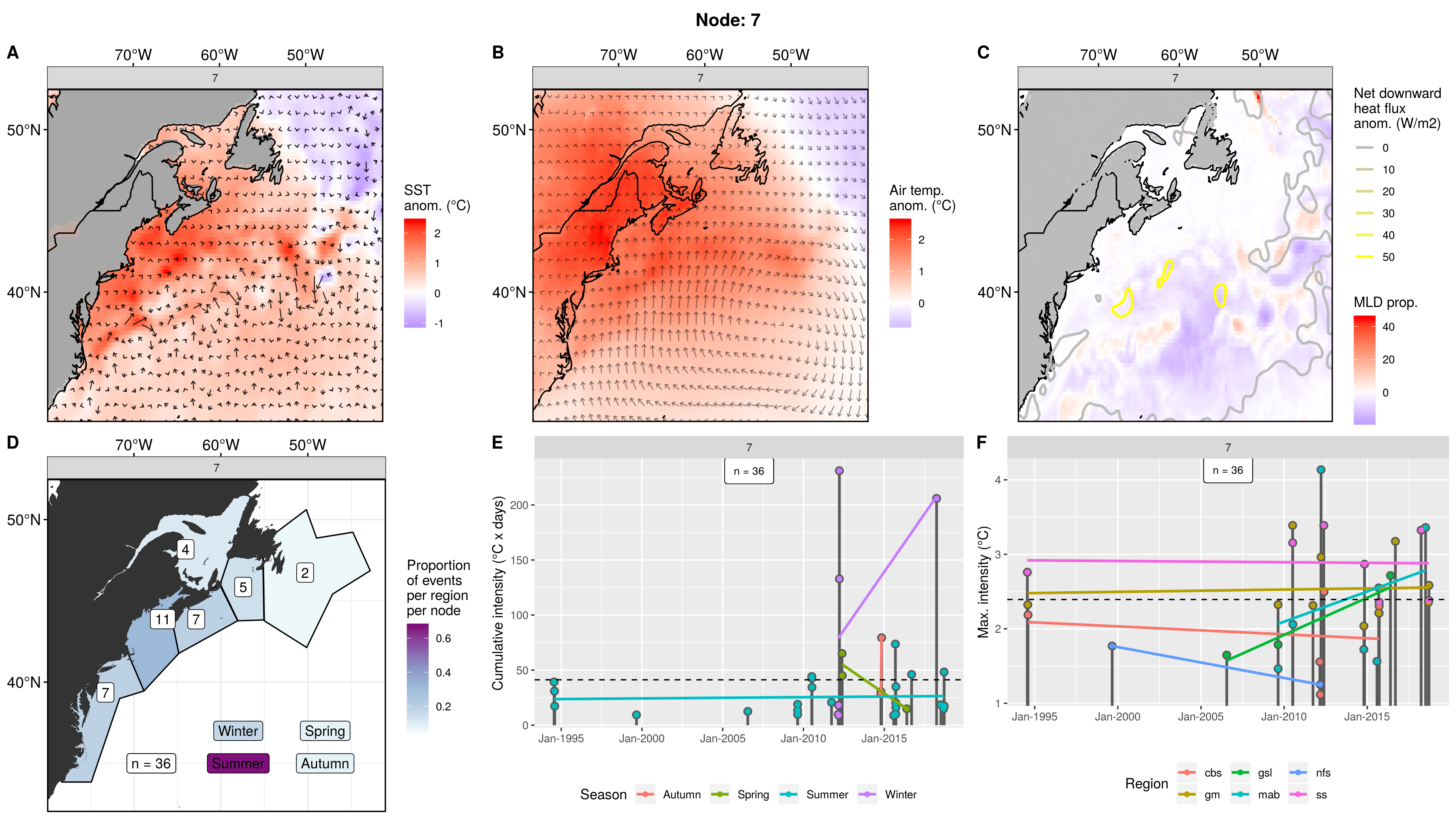
Expand here to see past versions of node_7_panels.png:
| Version | Author | Date |
|---|---|---|
| 9273f18 | robwschlegel | 2019-08-11 |
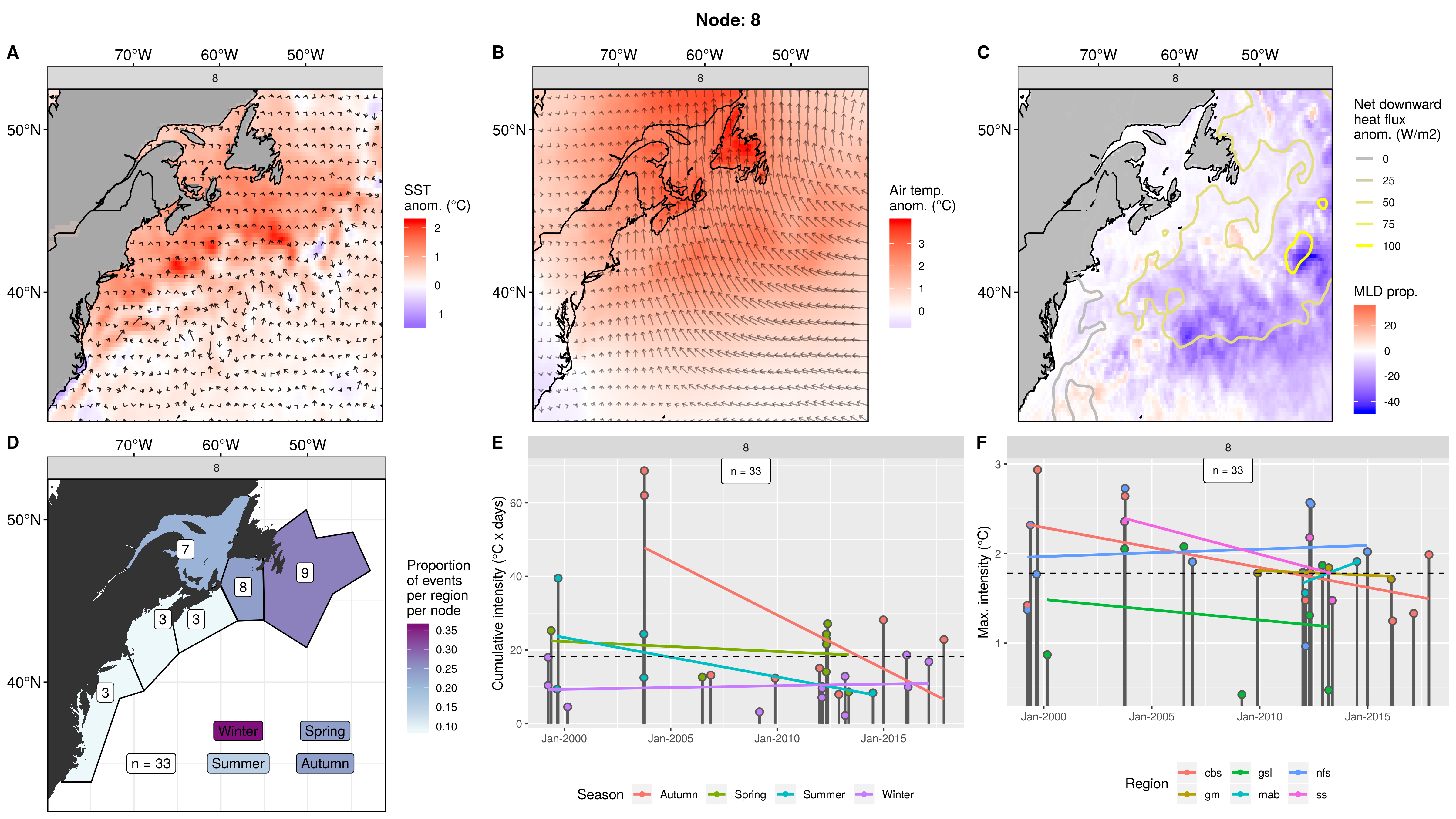
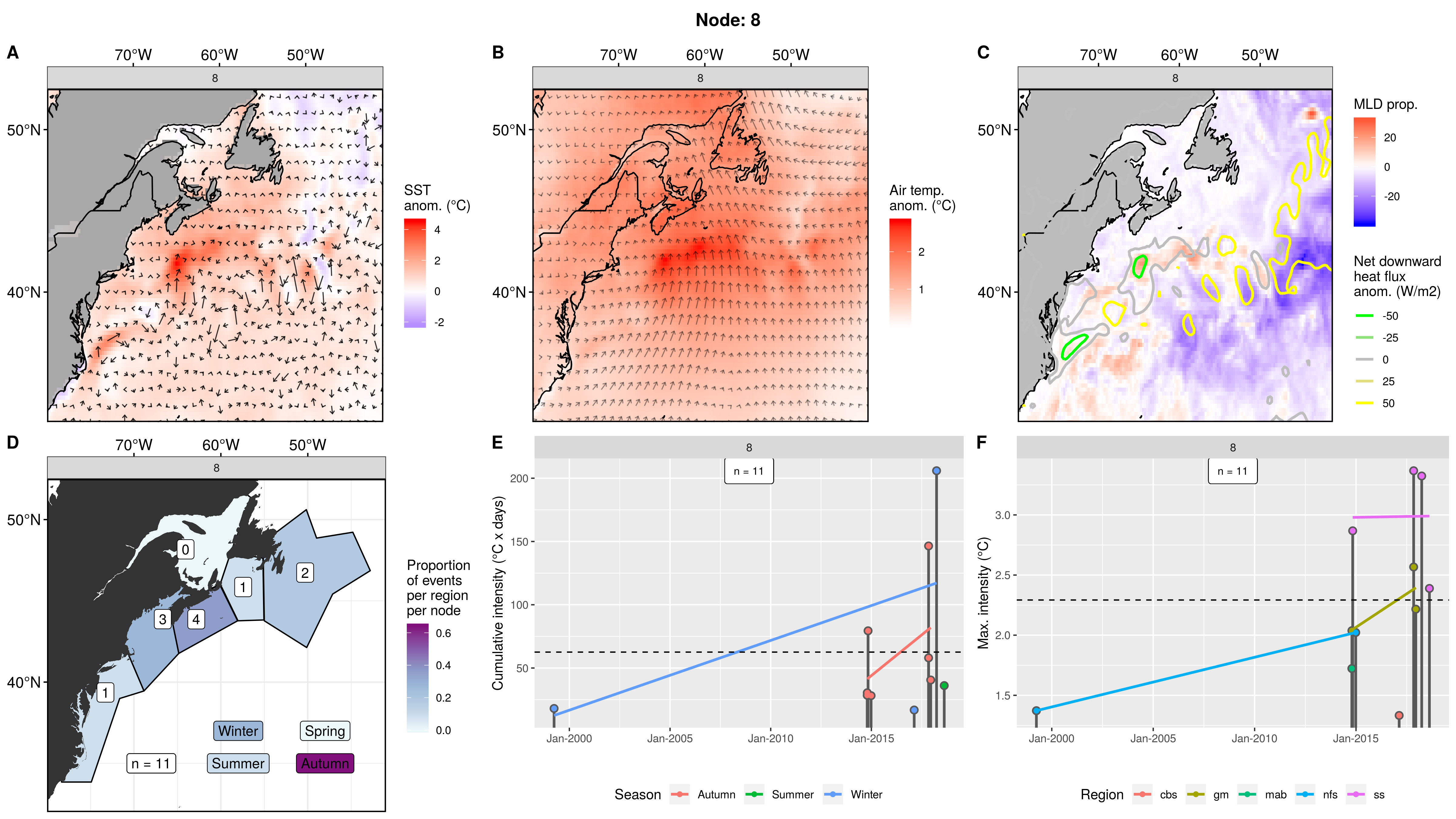
Node 8
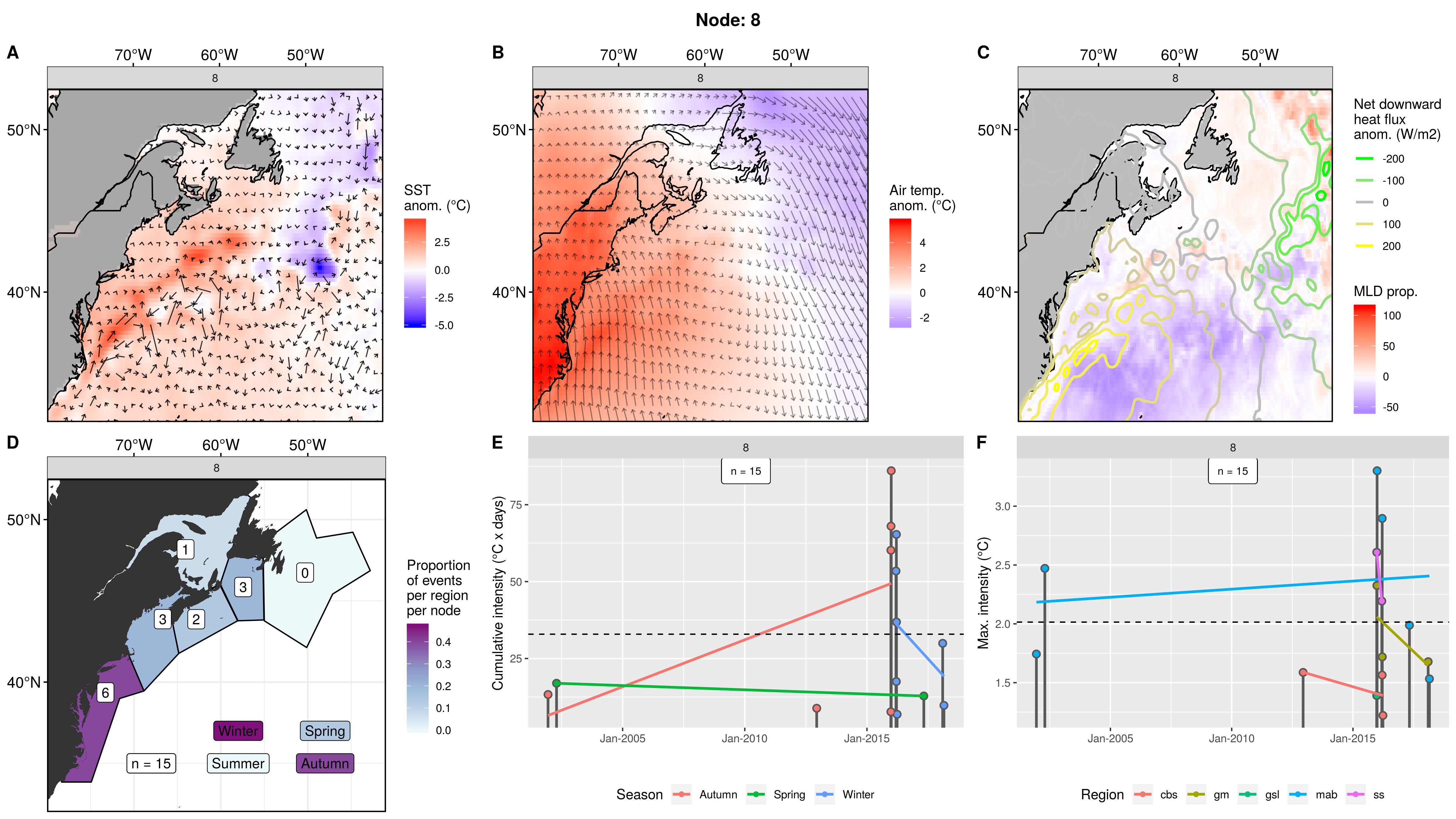
Expand here to see past versions of node_8_panels.png:
| Version | Author | Date |
|---|---|---|
| 9273f18 | robwschlegel | 2019-08-11 |
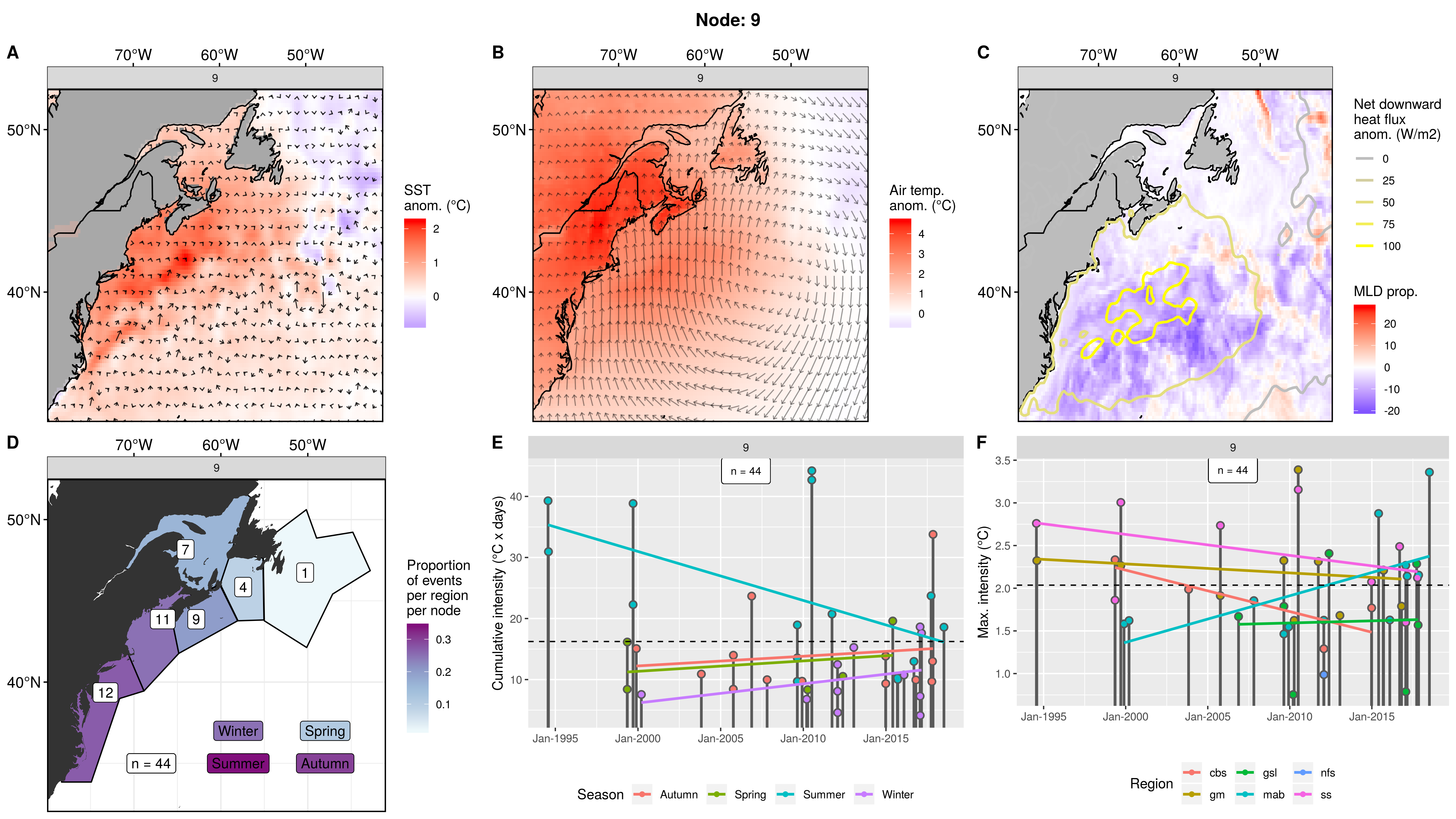
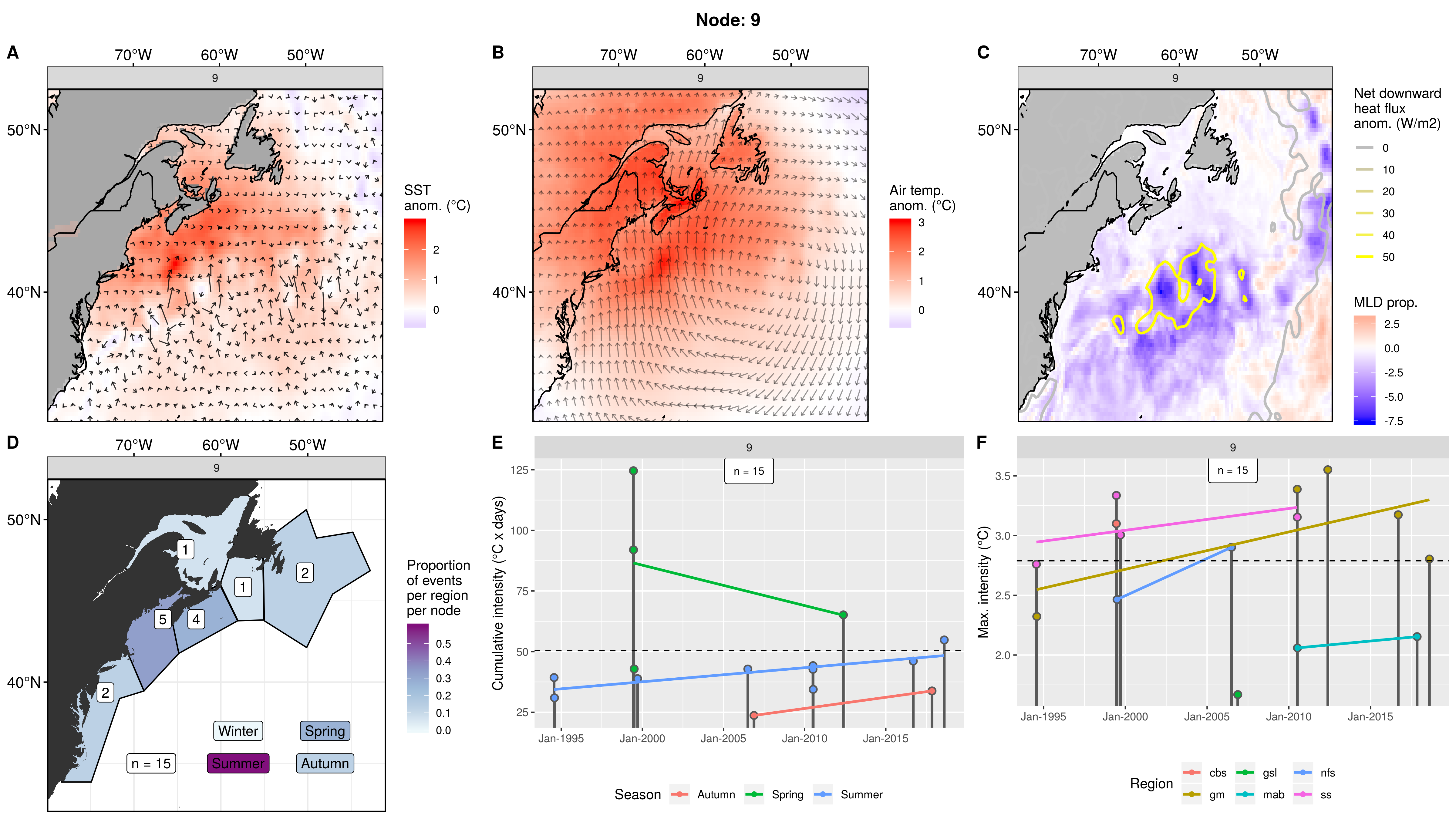
Node 9
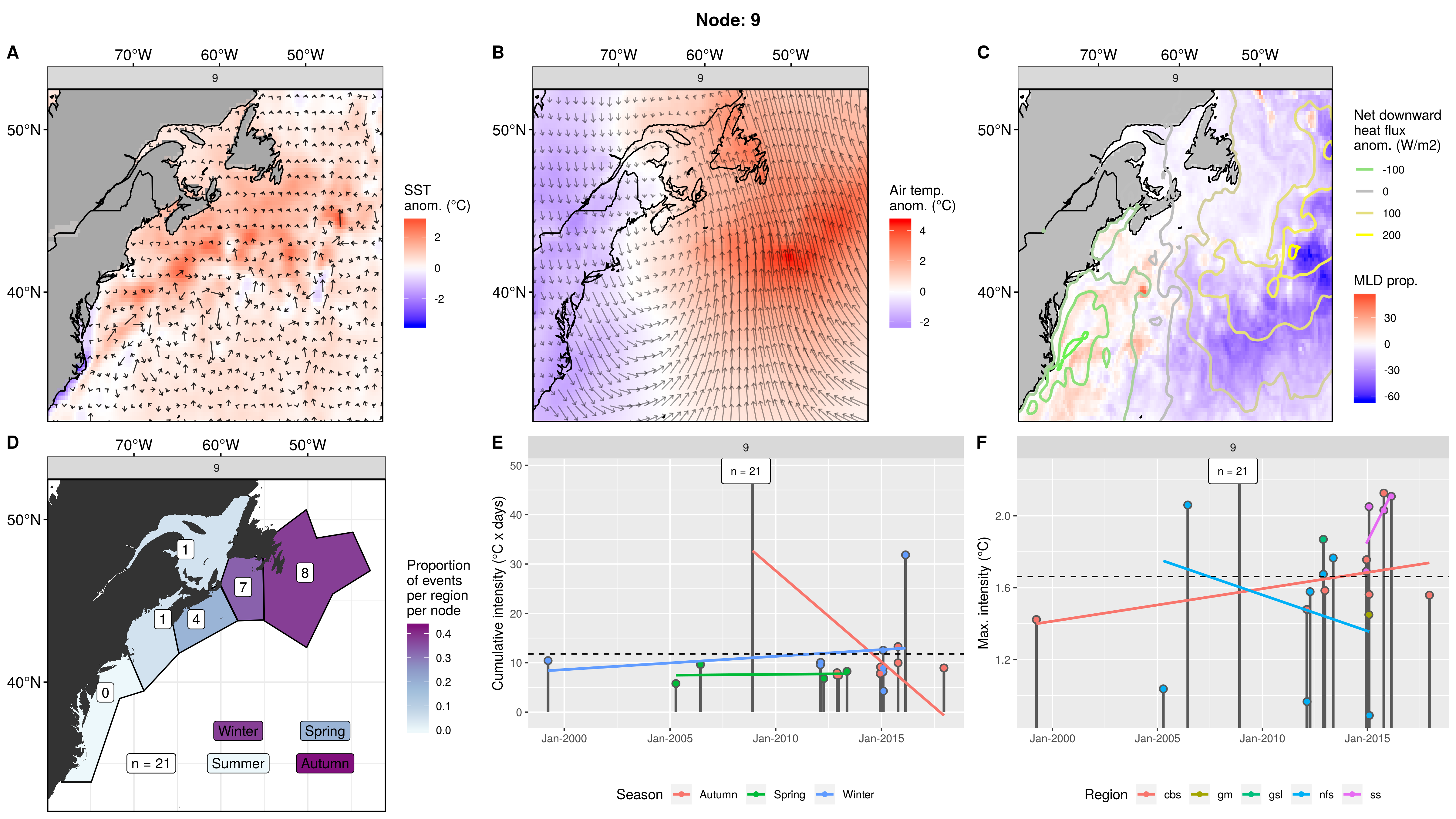
Expand here to see past versions of node_9_panels.png:
| Version | Author | Date |
|---|---|---|
| 9273f18 | robwschlegel | 2019-08-11 |
Node 10
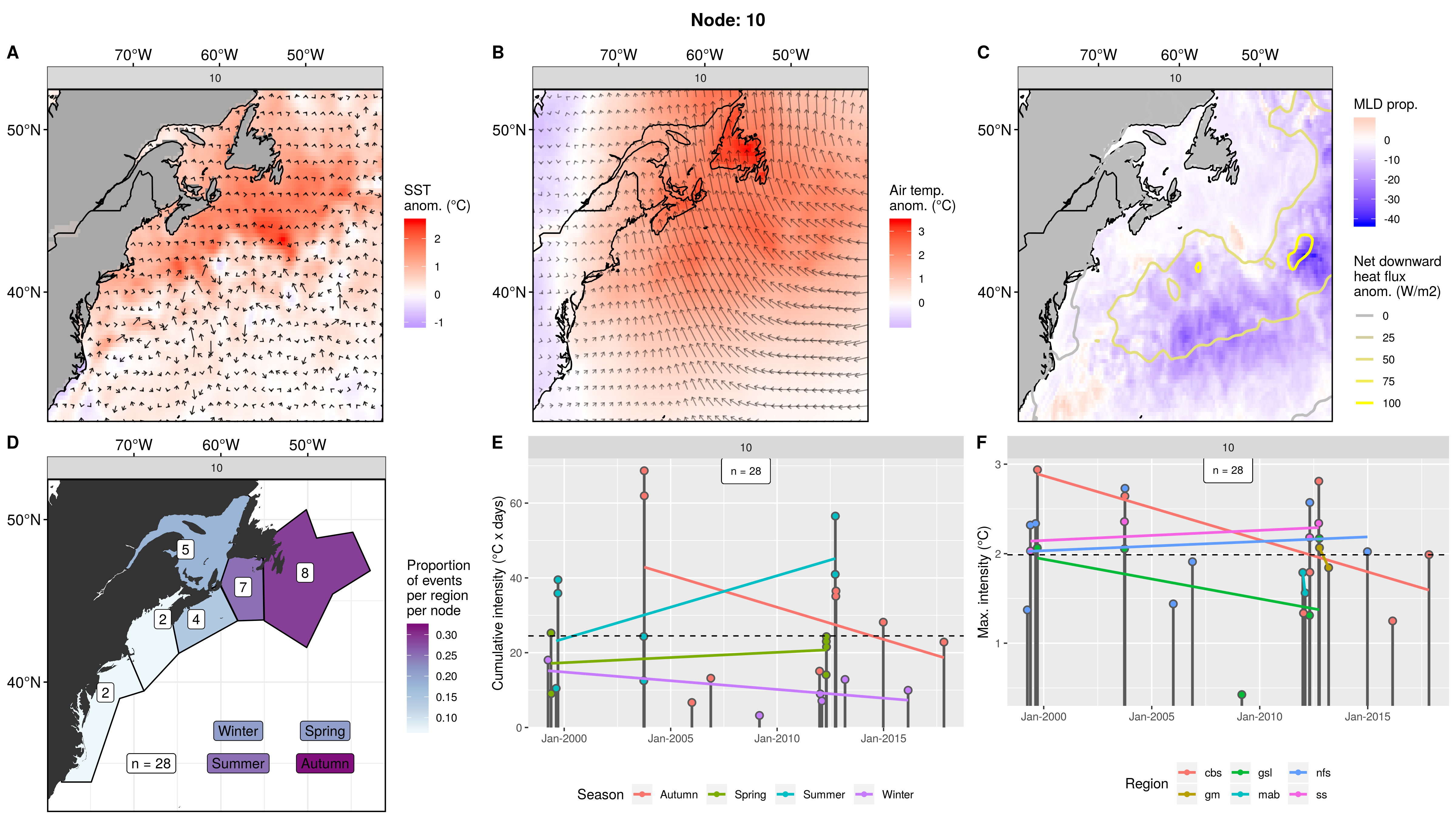
Expand here to see past versions of node_10_panels.png:
| Version | Author | Date |
|---|---|---|
| 9273f18 | robwschlegel | 2019-08-11 |
Node 11
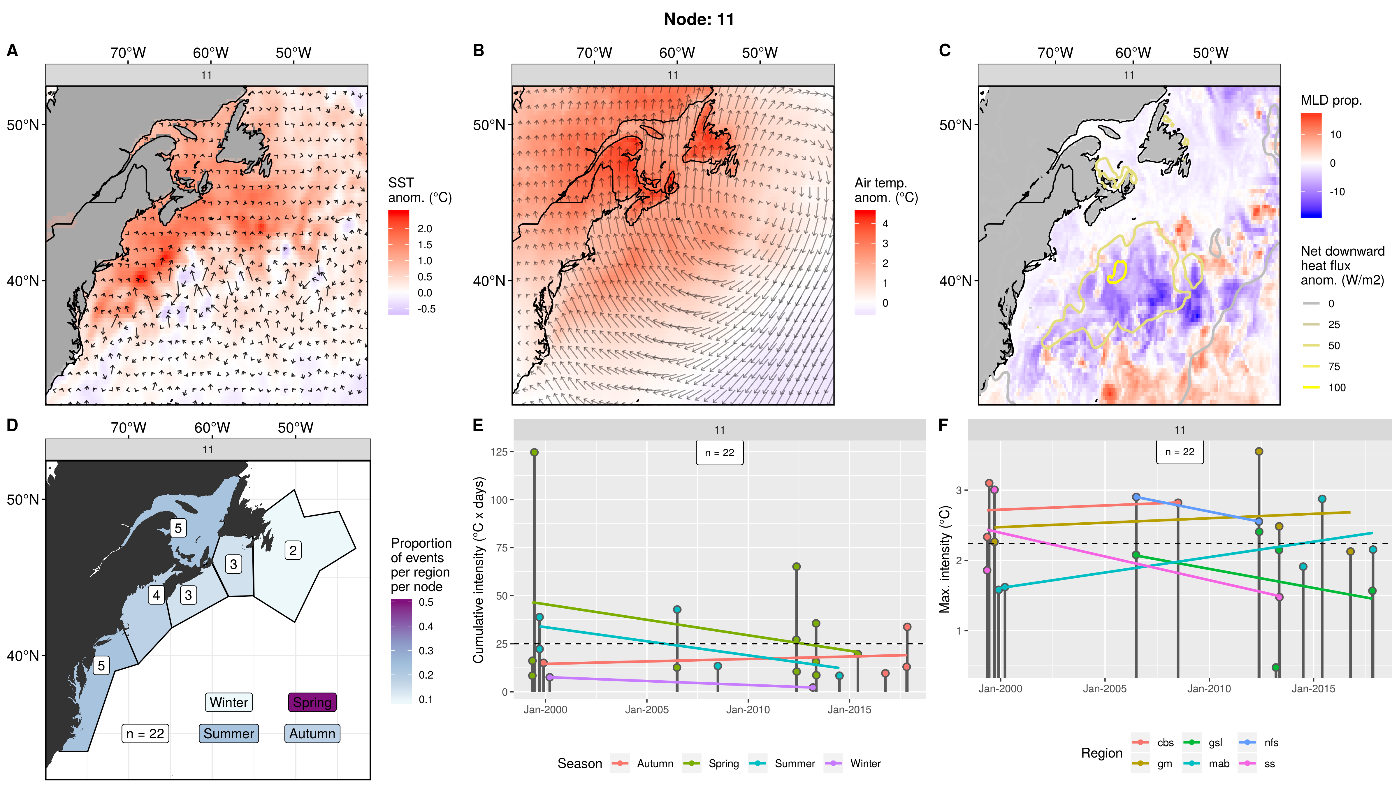
Expand here to see past versions of node_11_panels.png:
| Version | Author | Date |
|---|---|---|
| 9273f18 | robwschlegel | 2019-08-11 |
Node 12
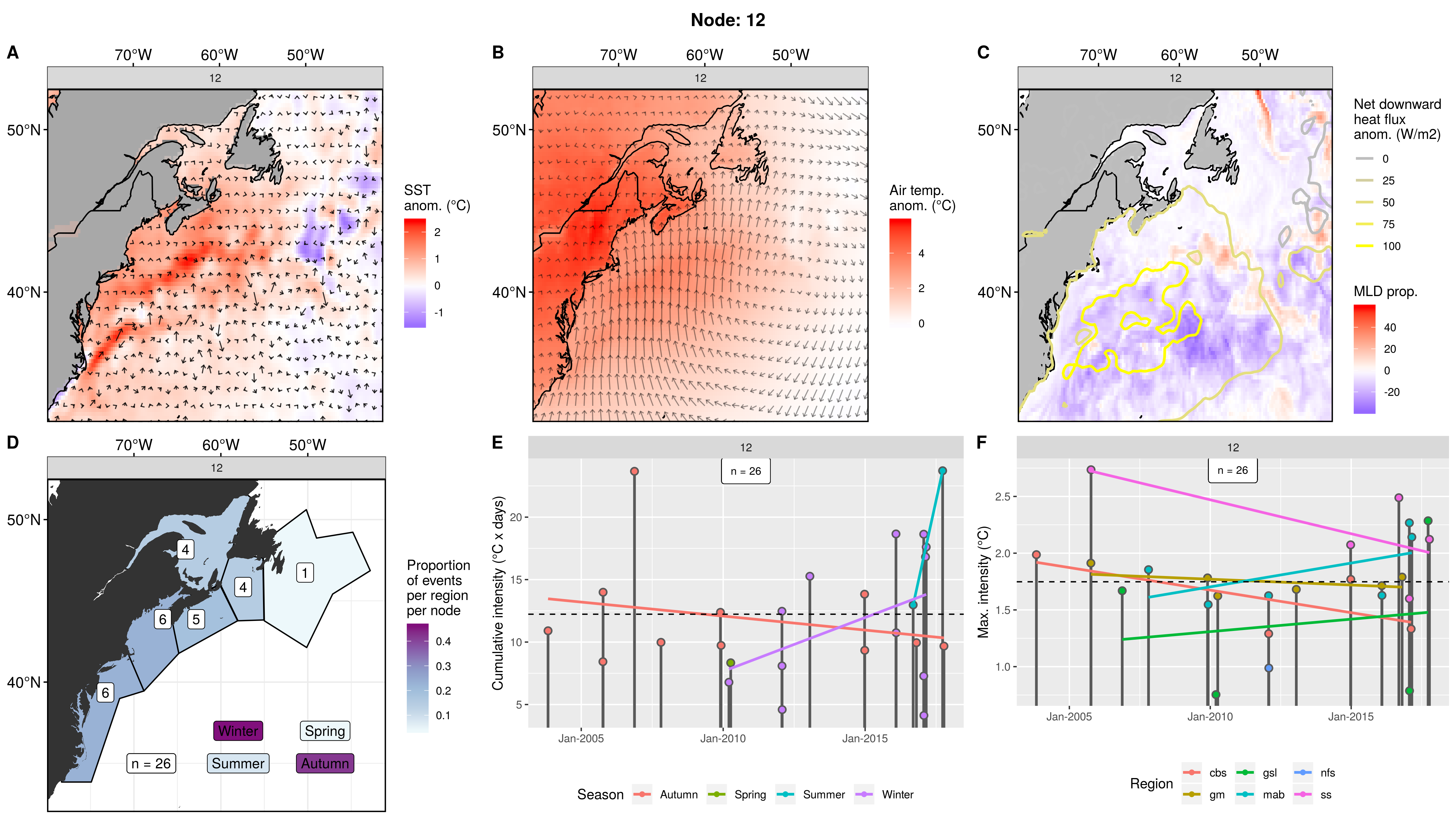
Expand here to see past versions of node_12_panels.png:
| Version | Author | Date |
|---|---|---|
| 9273f18 | robwschlegel | 2019-08-11 |
SOM experiment: Default, 3x3 nodes
Node summary table
The table below contains a concise summary of the nodes following Table 4 in Oliver et al. (2018). The following sub-sections provide more in-depth explanations.
| Node | Region | Season | MHW Properties | Conditions |
|---|---|---|---|---|
| 1 |
Season + region
Expand here to see past versions of fig_5.png:
| Version | Author | Date |
|---|---|---|
| 9273f18 | robwschlegel | 2019-08-11 |
SST + U + V
Expand here to see past versions of fig_2.png:
| Version | Author | Date |
|---|---|---|
| 9273f18 | robwschlegel | 2019-08-11 |
Air temp + U + V
Expand here to see past versions of fig_3.png:
| Version | Author | Date |
|---|---|---|
| 9273f18 | robwschlegel | 2019-08-11 |
MLD + Net downward heatflux
Expand here to see past versions of fig_4.png:
| Version | Author | Date |
|---|---|---|
| 9273f18 | robwschlegel | 2019-08-11 |
Node 1
Expand here to see past versions of node_1_panels.png:
| Version | Author | Date |
|---|---|---|
| 9273f18 | robwschlegel | 2019-08-11 |
Node 2
Expand here to see past versions of node_2_panels.png:
| Version | Author | Date |
|---|---|---|
| 9273f18 | robwschlegel | 2019-08-11 |
Node 3
Expand here to see past versions of node_3_panels.png:
| Version | Author | Date |
|---|---|---|
| 9273f18 | robwschlegel | 2019-08-11 |
Node 4
Expand here to see past versions of node_4_panels.png:
| Version | Author | Date |
|---|---|---|
| 9273f18 | robwschlegel | 2019-08-11 |
Node 5
Expand here to see past versions of node_5_panels.png:
| Version | Author | Date |
|---|---|---|
| 9273f18 | robwschlegel | 2019-08-11 |
Node 6
Expand here to see past versions of node_6_panels.png:
| Version | Author | Date |
|---|---|---|
| 9273f18 | robwschlegel | 2019-08-11 |
Node 7
Expand here to see past versions of node_7_panels.png:
| Version | Author | Date |
|---|---|---|
| 9273f18 | robwschlegel | 2019-08-11 |
Node 8
Expand here to see past versions of node_8_panels.png:
| Version | Author | Date |
|---|---|---|
| 9273f18 | robwschlegel | 2019-08-11 |
Node 9
Expand here to see past versions of node_9_panels.png:
| Version | Author | Date |
|---|---|---|
| 9273f18 | robwschlegel | 2019-08-11 |
SOM experiment: Default, no events under 14 days, 3x3 nodes
Node summary table
The table below contains a concise summary of the nodes following Table 4 in Oliver et al. (2018). The following sub-sections provide more in-depth explanations.
| Node | Region | Season | MHW Properties | Conditions |
|---|---|---|---|---|
| 1 |
Season + region
Expand here to see past versions of fig_5.png:
| Version | Author | Date |
|---|---|---|
| 9273f18 | robwschlegel | 2019-08-11 |
SST + U + V
Expand here to see past versions of fig_2.png:
| Version | Author | Date |
|---|---|---|
| 9273f18 | robwschlegel | 2019-08-11 |
Air temp + U + V
Expand here to see past versions of fig_3.png:
| Version | Author | Date |
|---|---|---|
| 9273f18 | robwschlegel | 2019-08-11 |
MLD + Net downward heatflux
Expand here to see past versions of fig_4.png:
| Version | Author | Date |
|---|---|---|
| 9273f18 | robwschlegel | 2019-08-11 |
Node 1
Expand here to see past versions of node_1_panels.png:
| Version | Author | Date |
|---|---|---|
| 9273f18 | robwschlegel | 2019-08-11 |
Node 2
Expand here to see past versions of node_2_panels.png:
| Version | Author | Date |
|---|---|---|
| 9273f18 | robwschlegel | 2019-08-11 |
Node 3
Expand here to see past versions of node_3_panels.png:
| Version | Author | Date |
|---|---|---|
| 9273f18 | robwschlegel | 2019-08-11 |
Node 4
Expand here to see past versions of node_4_panels.png:
| Version | Author | Date |
|---|---|---|
| 9273f18 | robwschlegel | 2019-08-11 |
Node 5
Expand here to see past versions of node_5_panels.png:
| Version | Author | Date |
|---|---|---|
| 9273f18 | robwschlegel | 2019-08-11 |
Node 6
Expand here to see past versions of node_6_panels.png:
| Version | Author | Date |
|---|---|---|
| 9273f18 | robwschlegel | 2019-08-11 |
Node 7
Expand here to see past versions of node_7_panels.png:
| Version | Author | Date |
|---|---|---|
| 9273f18 | robwschlegel | 2019-08-11 |
Node 8
Expand here to see past versions of node_8_panels.png:
| Version | Author | Date |
|---|---|---|
| 9273f18 | robwschlegel | 2019-08-11 |
Node 9
Expand here to see past versions of node_9_panels.png:
| Version | Author | Date |
|---|---|---|
| 9273f18 | robwschlegel | 2019-08-11 |
References
Oliver, E. C., Lago, V., Hobday, A. J., Holbrook, N. J., Ling, S. D., and Mundy, C. N. (2018). Marine heatwaves off eastern tasmania: Trends, interannual variability, and predictability. Progress in oceanography 161, 116–130.
Richaud, B., Kwon, Y.-O., Joyce, T. M., Fratantoni, P. S., and Lentz, S. J. (2016). Surface and bottom temperature and salinity climatology along the continental shelf off the canadian and us east coasts. Continental Shelf Research 124, 165–181.
Session information
R version 3.6.1 (2019-07-05)
Platform: x86_64-pc-linux-gnu (64-bit)
Running under: Ubuntu 16.04.5 LTS

Matrix products: default
BLAS:   /usr/lib/openblas-base/libblas.so.3
LAPACK: /usr/lib/libopenblasp-r0.2.18.so

locale:
 [1] LC_CTYPE=en_CA.UTF-8       LC_NUMERIC=C
 [3] LC_TIME=en_CA.UTF-8        LC_COLLATE=en_CA.UTF-8
 [5] LC_MONETARY=en_CA.UTF-8    LC_MESSAGES=en_CA.UTF-8
 [7] LC_PAPER=en_CA.UTF-8       LC_NAME=C
 [9] LC_ADDRESS=C               LC_TELEPHONE=C
[11] LC_MEASUREMENT=en_CA.UTF-8 LC_IDENTIFICATION=C

attached base packages:
[1] stats     graphics  grDevices utils     datasets  methods   base

loaded via a namespace (and not attached):
 [1] workflowr_1.1.1   Rcpp_0.12.18      digest_0.6.16
 [4] rprojroot_1.3-2   R.methodsS3_1.7.1 backports_1.1.2
 [7] git2r_0.23.0      magrittr_1.5      evaluate_0.11
[10] highr_0.7         stringi_1.2.4     whisker_0.3-2
[13] R.oo_1.22.0       R.utils_2.7.0     rmarkdown_1.10
[16] tools_3.6.1       stringr_1.3.1     yaml_2.2.0
[19] compiler_3.6.1    htmltools_0.3.6   knitr_1.20
This reproducible R Markdown analysis was created with workflowr 1.1.1