Comparing with mean (with signal)
Yuxin Zou
2018-01-11
Last updated: 2018-04-26
Loading required package: ashrcorrplot 0.84 loadedThe data contains 10 conditions with 10% non-null samples. For the non-null samples, it has equal effects in the first c conditions.
Let L be the contrast matrix that subtract mean from each sample.
\[\hat{\delta}_{j}|\delta_{j} \sim N(\delta_{j}, \frac{1}{2}LL')\] 90% of the true deviations are 0. 10% of the deviation \(\delta_{j}\) has correlation that the first c conditions are negatively correlated with the rest conditions.
Mash contrast model
We set \(c = 2\).
set.seed(1)
R = 10
C = 2
data = sim.mean.sig(nsamp=10000, ncond=C)
L = matrix(-1/R, R, R)
L[cbind(1:R,1:R)] = (R-1)/R
L.10 = L[1:(R-1),]
row.names(L.10) = seq(1,R-1)
mash_data = mash_set_data(Bhat=data$Chat, Shat=data$Shat)
mash_data_L.10 = mash_set_data_contrast(mash_data, L.10)U.c = cov_canonical(mash_data_L.10)
# data driven
# select max
m.1by1 = mash_1by1(mash_data_L.10)
strong = get_significant_results(m.1by1,0.05)
# center Z
mash_data_L.center = mash_data_L.10
mash_data_L.center$Bhat = mash_data_L.10$Bhat/mash_data_L.10$Shat # obtain z
mash_data_L.center$Shat = matrix(1, nrow(mash_data_L.10$Bhat),ncol(mash_data_L.10$Bhat))
mash_data_L.center$Bhat = apply(mash_data_L.center$Bhat, 2, function(x) x - mean(x))
U.pca = cov_pca(mash_data_L.center,2,strong)
U.ed = cov_ed(mash_data_L.center, U.pca, strong)
mashcontrast.model.10 = mash(mash_data_L.10, c(U.c, U.ed), algorithm.version = 'R', verbose = FALSE)Using mashcommonbaseline, there are 288 discoveries. The covariance structure found here is:
barplot(get_estimated_pi(mashcontrast.model.10),las = 2, cex.names = 0.7)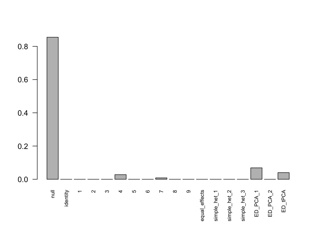 The correlation for PCA1 is:
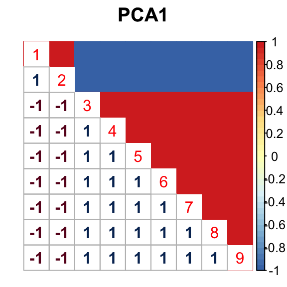
The correlation identified here is correct.
Subtract mean directly
If we subtract the mean from the data directly \[Var(\hat{c}_{j,r}-\bar{\hat{c}_{j}}) = \frac{1}{2} - \frac{1}{2R}\]
Indep.data.10 = mash_set_data(Bhat = mash_data_L.10$Bhat,
                           Shat = matrix(sqrt(0.5-1/(2*R)), nrow(data$Chat), R-1))

Indep.model.10 = mash(Indep.data.10, c(U.c, U.ed), algorithm.version = 'R', verbose = FALSE)
There are 336 discoveries, which is more than the mashcommonbaseline model. The covariance structure found here is:
barplot(get_estimated_pi(Indep.model.10),las = 2, cex.names = 0.7)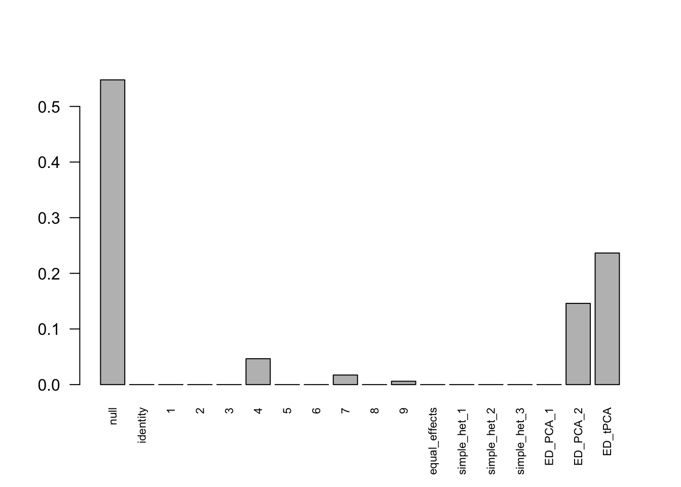 The weights for covariances are very different.
The correlation for PCA2 and tPCA is: 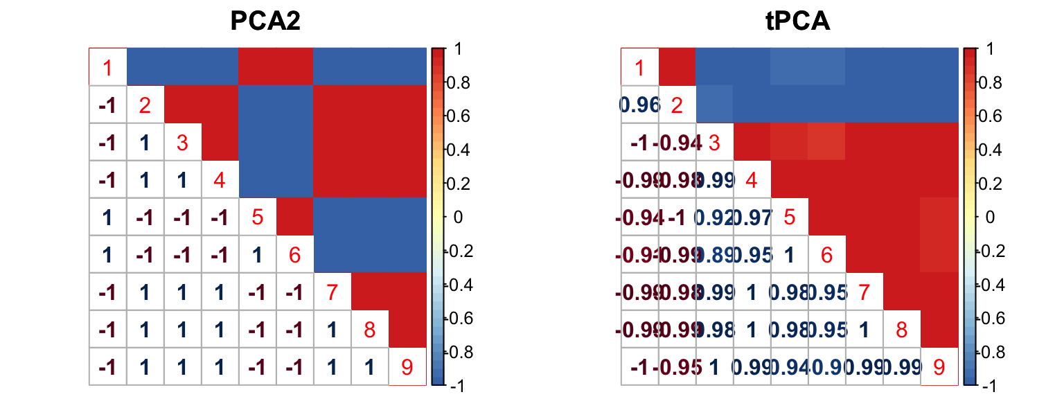
Compare models
The RRMSE plot:
delta = data$C %*% t(L.10)
barplot(c(sqrt(mean((delta - mashcontrast.model.10$result$PosteriorMean)^2)/mean((delta - data$Chat%*%t(L.10))^2)), sqrt(mean((delta - Indep.model.10$result$PosteriorMean)^2)/mean((delta - data$Chat%*%t(L.10))^2))), ylim=c(0,0.2), names.arg = c('mashcommonbaseline', 'mash.indep'), ylab='RRMSE')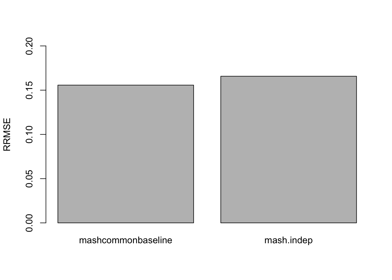
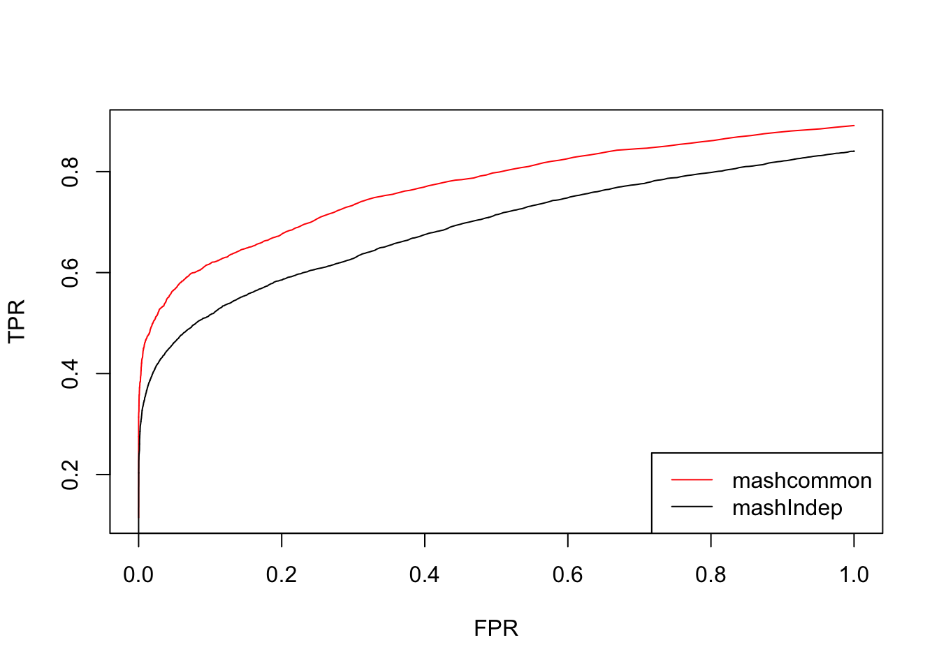
We check the False Positive Rate and True Positive Rate. \[FPR = \frac{|N\cap S|}{|N|} \quad TPR = \frac{|CS\cap S|}{|T|} \]
CS_S = function(model, thresh=0.05, data){
  sig.index = model$result$lfsr <= thresh
  sum(sig.index * model$result$PosteriorMean * data > 0)
}

N_S = function(model, thresh=0.05, data){
  N.index = data == 0
  sig.index = model$result$lfsr <= thresh
  sum(sig.index * N.index)
}

delta = data$C %*% t(L.10)
delta[abs(delta) <= 1e-14] = 0
N = sum(delta == 0)
Tr = nrow(delta) * ncol(delta) - N

thresh.seq = seq(0, 1, by=0.0005)[-1]
mashcontrast = matrix(0,length(thresh.seq), 2)
Indep = matrix(0,length(thresh.seq), 2)
colnames(mashcontrast) = c('TPR', 'FPR')
colnames(Indep) = c('TPR', 'FPR')
for(t in 1:length(thresh.seq)){
  mashcontrast[t,] = c(CS_S(mashcontrast.model.10, thresh.seq[t], delta)/Tr, N_S(mashcontrast.model.10, thresh.seq[t],delta)/N)
  Indep[t,] = c(CS_S(Indep.model.10, thresh.seq[t], delta)/Tr,  N_S(Indep.model.10, thresh.seq[t],delta)/N)
}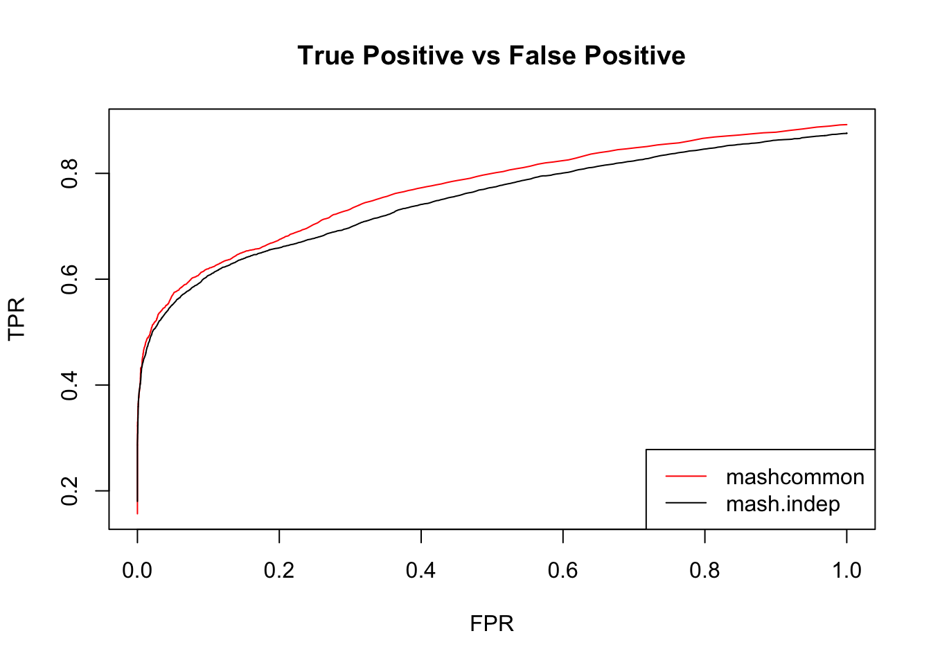
These methods are similar in terms of the number of false positives versus true positive. The mashcommonbaseline model is slightly better than mash.indep model.
Note:
The data was generated with signals in the first c conditions (\(c_{j,1}, \cdots, c_{j,c}\)). The contrast matrix L used here discards the last condition. The deviations are \(\hat{c}_{j,1} - \bar{\hat{c}_{j}}, \hat{c}_{j,2} - \bar{\hat{c}_{j}}, \cdots, \hat{c}_{j,R-1} - \bar{\hat{c}_{j}}\).
However, the contrast matrix L can discard any deviation from \(\hat{c}_{j,1} - \bar{\hat{c}_{j}}, \cdots, \hat{c}_{j,R} - \bar{\hat{c}_{j}}\). The choice of the discarded deviation could influence the reuslt.
We run the same model with L that discard the first deviation.
L.1 = L[2:R,]
row.names(L.1) = seq(2,R)
mash_data_L.1 = mash_set_data_contrast(mash_data, L.1)
U.c = cov_canonical(mash_data_L.1)
# data driven
# select max
m.1by1 = mash_1by1(mash_data_L.1)
strong = get_significant_results(m.1by1,0.05)
# center Z
mash_data_L.center = mash_data_L.1
mash_data_L.center$Bhat = mash_data_L.1$Bhat/mash_data_L.1$Shat # obtain z
mash_data_L.center$Shat = matrix(1, nrow(mash_data_L.1$Bhat),ncol(mash_data_L.1$Bhat))
mash_data_L.center$Bhat = apply(mash_data_L.center$Bhat, 2, function(x) x - mean(x))
U.pca = cov_pca(mash_data_L.center,2,strong)
U.ed = cov_ed(mash_data_L.center, U.pca, strong)
mashcontrast.model.1 = mash(mash_data_L.1, c(U.c, U.ed), algorithm.version = 'R', verbose = FALSE)Using mashcommonbaseline model, there are 283 discoveries. The covariance structure found here is:
barplot(get_estimated_pi(mashcontrast.model.1),las = 2, cex.names = 0.7)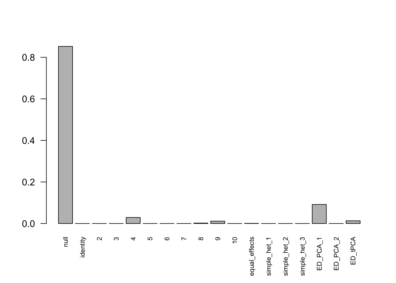 The correlation PCA 1 is:
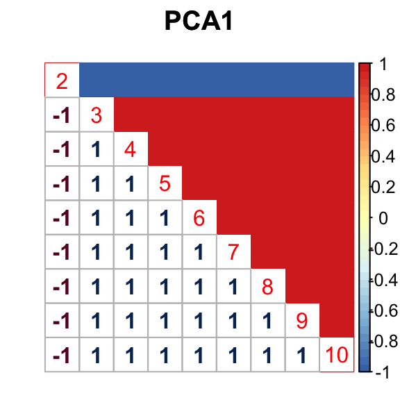
Indep.data.1 = mash_set_data(Bhat = mash_data_L.1$Bhat,
                           Shat = matrix(sqrt(0.5-1/(R*2)), nrow(data$Chat), R-1))

Indep.model.1 = mash(Indep.data.1, c(U.c, U.ed), algorithm.version = 'R', verbose = FALSE)
For mashIndep model, there are 217 discoveries, which is less than the mashcommonbaseline model. The covariance structure found here is:
barplot(get_estimated_pi(Indep.model.1),las = 2, cex.names = 0.7)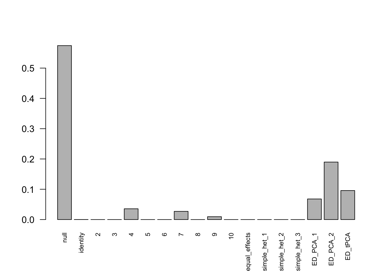
The correlation for PCA2 and tPCA is: 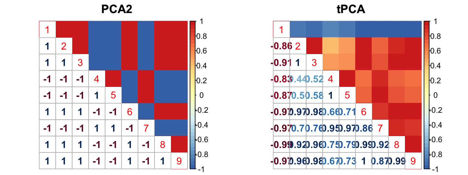
The RRMSE plot: 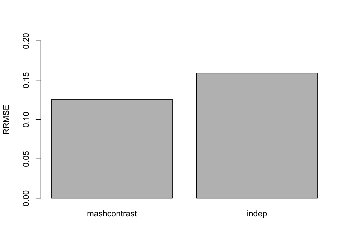
We check the False Positive Rate and True Positive Rate. \[FPR = \frac{|N\cap S|}{|N|} \quad TPR = \frac{|CS\cap S|}{|T|} \]
Using this contrast L, the results from mashcommonbaseline is much better than mashIndep.
Session information
sessionInfo()R version 3.4.4 (2018-03-15)
Platform: x86_64-apple-darwin15.6.0 (64-bit)
Running under: macOS High Sierra 10.13.4
Matrix products: default
BLAS: /Library/Frameworks/R.framework/Versions/3.4/Resources/lib/libRblas.0.dylib
LAPACK: /Library/Frameworks/R.framework/Versions/3.4/Resources/lib/libRlapack.dylib
locale:
[1] en_US.UTF-8/en_US.UTF-8/en_US.UTF-8/C/en_US.UTF-8/en_US.UTF-8
attached base packages:
[1] stats graphics grDevices utils datasets methods base
other attached packages:
[1] corrplot_0.84 mashr_0.2-6 ashr_2.2-7
loaded via a namespace (and not attached):
[1] Rcpp_0.12.16 knitr_1.20
[3] magrittr_1.5 REBayes_1.3
[5] MASS_7.3-49 doParallel_1.0.11
[7] pscl_1.5.2 SQUAREM_2017.10-1
[9] lattice_0.20-35 ExtremeDeconvolution_1.3
[11] foreach_1.4.4 plyr_1.8.4
[13] stringr_1.3.0 tools_3.4.4
[15] parallel_3.4.4 grid_3.4.4
[17] rmeta_3.0 htmltools_0.3.6
[19] iterators_1.0.9 assertthat_0.2.0
[21] yaml_2.1.18 rprojroot_1.3-2
[23] digest_0.6.15 Matrix_1.2-14
[25] codetools_0.2-15 evaluate_0.10.1
[27] rmarkdown_1.9 stringi_1.1.7
[29] compiler_3.4.4 Rmosek_8.0.69
[31] backports_1.1.2 mvtnorm_1.0-7
[33] truncnorm_1.0-8 This R Markdown site was created with workflowr