Estimate Null Correlation Problem
Yuxin Zou
2018-07-09
Last updated: 2018-08-20
workflowr checks: (Click a bullet for more information)-
✔ R Markdown file: up-to-date
Great! Since the R Markdown file has been committed to the Git repository, you know the exact version of the code that produced these results.
-
✔ Environment: empty
Great job! The global environment was empty. Objects defined in the global environment can affect the analysis in your R Markdown file in unknown ways. For reproduciblity it’s best to always run the code in an empty environment.
-
✔ Seed:
set.seed(1)The command
set.seed(1)was run prior to running the code in the R Markdown file. Setting a seed ensures that any results that rely on randomness, e.g. subsampling or permutations, are reproducible. -
✔ Session information: recorded
Great job! Recording the operating system, R version, and package versions is critical for reproducibility.
-
Great! You are using Git for version control. Tracking code development and connecting the code version to the results is critical for reproducibility. The version displayed above was the version of the Git repository at the time these results were generated.✔ Repository version: a80bf6f
Note that you need to be careful to ensure that all relevant files for the analysis have been committed to Git prior to generating the results (you can usewflow_publishorwflow_git_commit). workflowr only checks the R Markdown file, but you know if there are other scripts or data files that it depends on. Below is the status of the Git repository when the results were generated:
Note that any generated files, e.g. HTML, png, CSS, etc., are not included in this status report because it is ok for generated content to have uncommitted changes.Ignored files: Ignored: .DS_Store Ignored: .Rhistory Ignored: .Rproj.user/ Ignored: analysis/.DS_Store Ignored: analysis/.Rhistory Ignored: analysis/figure/ Ignored: analysis/include/.DS_Store Ignored: data/.DS_Store Ignored: docs/.DS_Store Ignored: output/.DS_Store Untracked files: Untracked: _workflowr.yml Untracked: analysis/Classify.Rmd Untracked: analysis/EstimateCorMaxEM.Rmd Untracked: analysis/EstimateCorMaxEMGD.Rmd Untracked: analysis/EstimateCorPrior.Rmd Untracked: analysis/EstimateCorSol.Rmd Untracked: analysis/HierarchicalFlashSim.Rmd Untracked: analysis/MashLowSignal.Rmd Untracked: analysis/Mash_GTEx.Rmd Untracked: analysis/MeanAsh.Rmd Untracked: analysis/OutlierDetection.Rmd Untracked: analysis/OutlierDetection2.Rmd Untracked: analysis/OutlierDetection3.Rmd Untracked: analysis/OutlierDetection4.Rmd Untracked: analysis/Test.Rmd Untracked: analysis/mash_missing_row.Rmd Untracked: code/MashClassify.R Untracked: code/MashCorResult.R Untracked: code/MashSource.R Untracked: code/Weight_plot.R Untracked: code/addemV.R Untracked: code/estimate_cor.R Untracked: code/generateDataV.R Untracked: code/johnprocess.R Untracked: code/sim_mean_sig.R Untracked: code/summary.R Untracked: data/Blischak_et_al_2015/ Untracked: data/scale_data.rds Untracked: docs/figure/Classify.Rmd/ Untracked: docs/figure/OutlierDetection.Rmd/ Untracked: docs/figure/OutlierDetection2.Rmd/ Untracked: docs/figure/OutlierDetection3.Rmd/ Untracked: docs/figure/Test.Rmd/ Untracked: docs/figure/mash_missing_whole_row_5.Rmd/ Untracked: docs/include/ Untracked: output/AddEMV/ Untracked: output/CovED_UKBio_strong.rds Untracked: output/CovED_UKBio_strong_Z.rds Untracked: output/Flash_UKBio_strong.rds Untracked: output/MASH.10.em2.result.rds Untracked: output/MASH.10.mle.result.rds Untracked: output/MASH.result.1.rds Untracked: output/MASH.result.10.rds Untracked: output/MASH.result.2.rds Untracked: output/MASH.result.3.rds Untracked: output/MASH.result.4.rds Untracked: output/MASH.result.5.rds Untracked: output/MASH.result.6.rds Untracked: output/MASH.result.7.rds Untracked: output/MASH.result.8.rds Untracked: output/MASH.result.9.rds Untracked: output/Mash_EE_Cov_0_plusR1.rds Untracked: output/Trail 1/ Untracked: output/Trail 2/ Untracked: output/UKBio_mash_model.rds Unstaged changes: Modified: analysis/EstimateCorMaxEM2.Rmd Modified: analysis/EstimateCorMaxMash.Rmd Modified: analysis/Mash_UKBio.Rmd Modified: analysis/_site.yml Modified: analysis/chunks.R Modified: analysis/mash_missing_samplesize.Rmd Modified: output/Flash_T2_0.rds Modified: output/Flash_T2_0_mclust.rds Modified: output/Mash_model_0_plusR1.rds Modified: output/PresiAddVarCol.rds
Expand here to see past versions:
| File | Version | Author | Date | Message |
|---|---|---|---|---|
| Rmd | a80bf6f | zouyuxin | 2018-08-20 | wflow_publish(“analysis/EstimateCor.Rmd”) |
| html | 6281062 | zouyuxin | 2018-08-15 | Build site. |
| Rmd | 3e3e128 | zouyuxin | 2018-08-15 | wflow_publish(c(“analysis/EstimateCor.Rmd”, “analysis/EstimateCorMax.Rmd”, |
| html | 05731eb | zouyuxin | 2018-08-15 | Build site. |
| Rmd | ccc1607 | zouyuxin | 2018-08-15 | wflow_publish(c(“analysis/EstimateCorIndex.Rmd”, “analysis/EstimateCor.Rmd”)) |
| html | 568fbe6 | zouyuxin | 2018-08-13 | Build site. |
| Rmd | 3ae3f08 | zouyuxin | 2018-08-13 | wflow_publish(c(“analysis/EstimateCor.Rmd”, |
| html | 10d4174 | zouyuxin | 2018-08-13 | Build site. |
| Rmd | b8c1cd8 | zouyuxin | 2018-08-13 | wflow_publish(“analysis/EstimateCor.Rmd”) |
| html | 3bfa4f5 | zouyuxin | 2018-08-13 | Build site. |
| Rmd | 49d53fb | zouyuxin | 2018-08-13 | wflow_publish(“analysis/EstimateCor.Rmd”) |
| html | 6e4f0a1 | zouyuxin | 2018-08-03 | Build site. |
| Rmd | c330f07 | zouyuxin | 2018-08-03 | wflow_publish(c(“analysis/EstimateCor.Rmd”)) |
| html | 2985466 | zouyuxin | 2018-07-26 | Build site. |
| Rmd | e2c5ebd | zouyuxin | 2018-07-26 | wflow_publish(“analysis/EstimateCor.Rmd”) |
library(mashr)Loading required package: ashrlibrary(knitr)
library(kableExtra)
source('../code/generateDataV.R')
source('../code/summary.R')We illustrate the problem about estimating the correlation matrix in mashr.
In my simple simulation, the current approach underestimates the null correlation. We want to find better positive definite estimator. We could try to estimate the pairwise correlation, ie. mle of \(\sum_{l,k} \pi_{lk} N_{2}(0, V + w_{l}U_{k})\) for any pair of conditions.
Problem
Simple simulation in \(R^2\) to illustrate the problem: \[ \hat{\beta}|\beta \sim N_{2}(\hat{\beta}; \beta, \left(\begin{matrix} 1 & 0.5 \\ 0.5 & 1 \end{matrix}\right)) \]
\[ \beta \sim \frac{1}{4}\delta_{0} + \frac{1}{4}N_{2}(0, \left(\begin{matrix} 1 & 0 \\ 0 & 0 \end{matrix}\right)) + \frac{1}{4}N_{2}(0, \left(\begin{matrix} 0 & 0 \\ 0 & 1 \end{matrix}\right)) + \frac{1}{4}N_{2}(0, \left(\begin{matrix} 1 & 1 \\ 1 & 1 \end{matrix}\right)) \]
\(\Rightarrow\) \[ \hat{\beta} \sim \frac{1}{4}N_{2}(0, \left( \begin{matrix} 1 & 0.5 \\ 0.5 & 1 \end{matrix} \right)) + \frac{1}{4}N_{2}(0, \left( \begin{matrix} 2 & 0.5 \\ 0.5 & 1 \end{matrix} \right)) + \frac{1}{4}N_{2}(0, \left( \begin{matrix} 1 & 0.5 \\ 0.5 & 2 \end{matrix} \right)) + \frac{1}{4}N_{2}(0, \left( \begin{matrix} 2 & 1.5 \\ 1.5 & 2 \end{matrix} \right)) \]
n = 4000
set.seed(1)
n = 4000; p = 2
Sigma = matrix(c(1,0.5,0.5,1),p,p)
U0 = matrix(0,2,2)
U1 = U0; U1[1,1] = 1
U2 = U0; U2[2,2] = 1
U3 = matrix(1,2,2)
Utrue = list(U0=U0, U1=U1, U2=U2, U3=U3)
data = generate_data(n, p, Sigma, Utrue)
Let’s check the result of mash under different correlation matrix:
- Identity \[ V.I = I_{2} \]
m.data = mash_set_data(data$Bhat, data$Shat)
U.c = cov_canonical(m.data)
m.I = mash(m.data, U.c, verbose= FALSE)- The current approach: truncated empirical correlation \(V.trun\)
Vhat = estimate_null_correlation(m.data, apply_lower_bound = FALSE)
Vhat
[,1] [,2]
[1,] 1.0000000 0.3439205
[2,] 0.3439205 1.0000000It underestimates the correlation.
# Use underestimate cor
m.data.V = mash_set_data(data$Bhat, data$Shat, V=Vhat)
m.V = mash(m.data.V, U.c, verbose = FALSE)- Overestimate correlation \[ V.o = \left( \begin{matrix} 1 & 0.65 \\ 0.65 & 1\end{matrix} \right) \]
# If we overestimate cor
V.o = matrix(c(1,0.65,0.65,1),2,2)
m.data.Vo = mash_set_data(data$Bhat, data$Shat, V=V.o)
m.Vo = mash(m.data.Vo, U.c, verbose=FALSE)- mash.1by1
We run ash for each condition, and estimate correlation matrix based on the non-significant genes. The estimated cor is closer to the truth.
m.1by1 = mash_1by1(m.data)
strong = get_significant_results(m.1by1)
V.mash = cor(data$Bhat[-strong,])
V.mash
[,1] [,2]
[1,] 1.0000000 0.4597745
[2,] 0.4597745 1.0000000m.data.1by1 = mash_set_data(data$Bhat, data$Shat, V=V.mash)
m.V1by1 = mash(m.data.1by1, U.c, verbose = FALSE)- True correlation
# With correct cor
m.data.correct = mash_set_data(data$Bhat, data$Shat, V=Sigma)
m.correct = mash(m.data.correct, U.c, verbose = FALSE)
The results are summarized in table:
null.ind = which(apply(data$B,1,sum) == 0)
V.trun = c(get_loglik(m.V), length(get_significant_results(m.V)), sum(get_significant_results(m.V) %in% null.ind))
V.I = c(get_loglik(m.I), length(get_significant_results(m.I)), sum(get_significant_results(m.I) %in% null.ind))
V.over = c(get_loglik(m.Vo), length(get_significant_results(m.Vo)), sum(get_significant_results(m.Vo) %in% null.ind))
V.1by1 = c(get_loglik(m.V1by1), length(get_significant_results(m.V1by1)), sum(get_significant_results(m.V1by1) %in% null.ind))
V.correct = c(get_loglik(m.correct), length(get_significant_results(m.correct)), sum(get_significant_results(m.correct) %in% null.ind))
temp = cbind(V.I, V.trun, V.1by1, V.correct, V.over)
colnames(temp) = c('Identity','truncate', 'm.1by1', 'true', 'overestimate')
row.names(temp) = c('log likelihood', '# significance', '# False positive')
temp %>% kable() %>% kable_styling()| Identity | truncate | m.1by1 | true | overestimate | |
|---|---|---|---|---|---|
| log likelihood | -12390.14 | -12307.65 | -12304.13 | -12302.62 | -12301.81 |
| # significance | 166.00 | 30.00 | 25.00 | 25.00 | 70.00 |
| # False positive | 14.00 | 1.00 | 0.00 | 0.00 | 4.00 |
The estimated pi is
par(mfrow=c(2,3))
barplot(get_estimated_pi(m.I), las=2, cex.names = 0.7, main='Identity', ylim=c(0,0.8))
barplot(get_estimated_pi(m.V), las=2, cex.names = 0.7, main='Truncate', ylim=c(0,0.8))
barplot(get_estimated_pi(m.V1by1), las=2, cex.names = 0.7, main='m.1by1', ylim=c(0,0.8))
barplot(get_estimated_pi(m.correct), las=2, cex.names = 0.7, main='True', ylim=c(0,0.8))
barplot(get_estimated_pi(m.Vo), las=2, cex.names = 0.7, main='OverEst', ylim=c(0,0.8))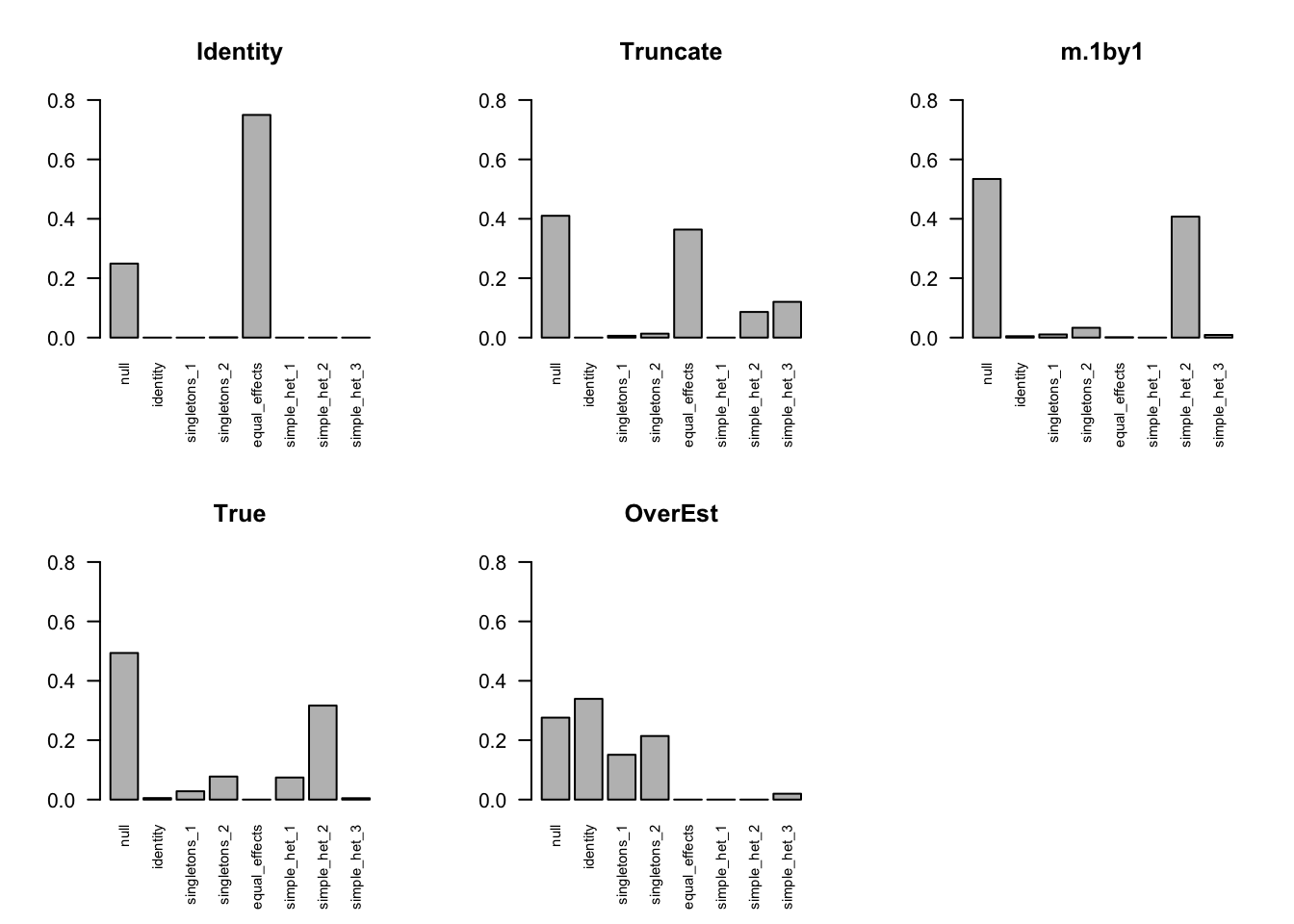
Expand here to see past versions of unnamed-chunk-10-1.png:
| Version | Author | Date |
|---|---|---|
| 10d4174 | zouyuxin | 2018-08-13 |
| 3bfa4f5 | zouyuxin | 2018-08-13 |
| 2985466 | zouyuxin | 2018-07-26 |
The ROC curve:
m.I.seq = ROC.table(data$B, m.I)
m.V.seq = ROC.table(data$B, m.V)
m.Vo.seq = ROC.table(data$B, m.Vo)
m.V1by1.seq = ROC.table(data$B, m.V1by1)
m.correct.seq = ROC.table(data$B, m.correct)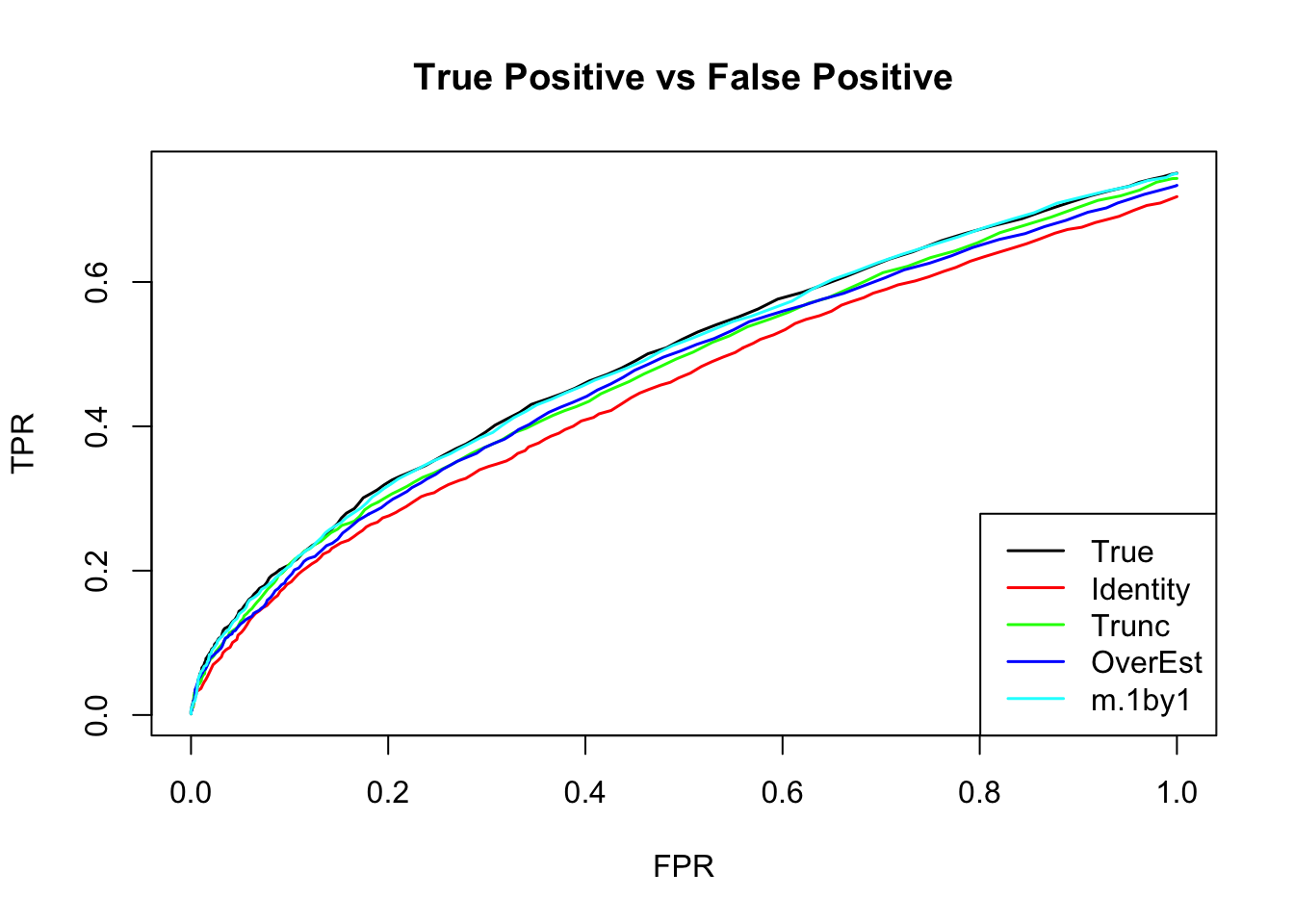
Expand here to see past versions of unnamed-chunk-12-1.png:
| Version | Author | Date |
|---|---|---|
| 10d4174 | zouyuxin | 2018-08-13 |
| 3bfa4f5 | zouyuxin | 2018-08-13 |
| 2985466 | zouyuxin | 2018-07-26 |
Comparing accuracy
rrmse = rbind(RRMSE(data$B, data$Bhat, list(m.I = m.I, m.V = m.V, m.1by1 = m.V1by1, m.true = m.correct, m.over = m.Vo)))
colnames(rrmse) = c('Identity','V.trun','V.1by1','V.true','V.over')
row.names(rrmse) = 'RRMSE'
rrmse %>% kable() %>% kable_styling()| Identity | V.trun | V.1by1 | V.true | V.over | |
|---|---|---|---|---|---|
| RRMSE | 0.6522463 | 0.5925754 | 0.5811472 | 0.5817699 | 0.6052702 |
barplot(rrmse, ylim=c(0,(1+max(rrmse))/2), las=2, cex.names = 0.7, main='RRMSE')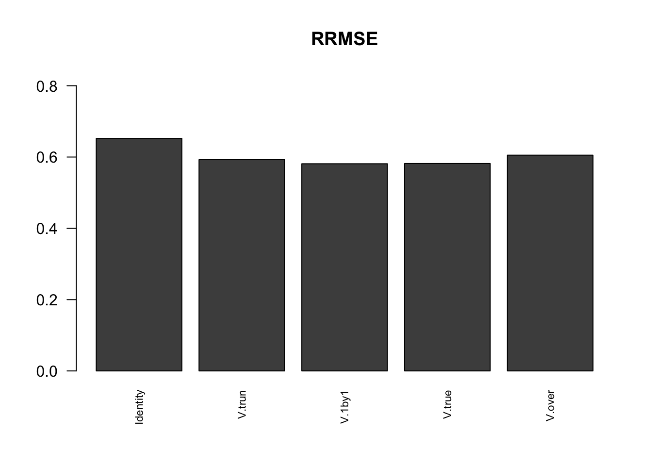
Solution: MLE
K=1
Suppose a simple extreme case \[ \left(\begin{matrix} \hat{x} \\ \hat{y} \end{matrix} \right)| \left(\begin{matrix} x \\ y \end{matrix} \right) \sim N_{2}(\left(\begin{matrix} \hat{x} \\ \hat{y} \end{matrix} \right); \left(\begin{matrix} x \\ y \end{matrix} \right), \left( \begin{matrix} 1 & \rho \\ \rho & 1 \end{matrix}\right)) \] \[ \left(\begin{matrix} x \\ y \end{matrix} \right) \sim \delta_{0} \] \(\Rightarrow\) \[ \left(\begin{matrix} \hat{x} \\ \hat{y} \end{matrix} \right) \sim N_{2}(\left(\begin{matrix} \hat{x} \\ \hat{y} \end{matrix} \right); \left(\begin{matrix} 0 \\ 0 \end{matrix} \right), \left( \begin{matrix} 1 & \rho \\ \rho & 1 \end{matrix}\right)) \]
\[ f(\hat{x},\hat{y}) = \prod_{i=1}^{n} \frac{1}{2\pi\sqrt{1-\rho^2}} \exp \{-\frac{1}{2(1-\rho^2)}\left[ \hat{x}_{i}^2 + \hat{y}_{i}^2 - 2\rho \hat{x}_{i}\hat{y}_{i}\right] \} \] The MLE of \(\rho\): \[ \begin{align*} l(\rho) &= -\frac{n}{2}\log(1-\rho^2) - \frac{1}{2(1-\rho^2)}\left( \sum_{i=1}^{n} x_{i}^2 + y_{i}^2 - 2\rho x_{i}y_{i} \right) \\ l(\rho)' &= \frac{n\rho}{1-\rho^2} - \frac{\rho}{(1-\rho^2)^2} \sum_{i=1}^{n} (x_{i}^2 + y_{i}^2) + \frac{\rho^2 + 1}{(1-\rho^2)^2} \sum_{i=1}^{n} x_{i}y_{i} = 0 \\ &= \rho^{3} - \rho^{2}\frac{1}{n}\sum_{i=1}^{n} x_{i}y_{i} - \left( 1- \frac{1}{n} \sum_{i=1}^{n} x_{i}^{2} + y_{i}^{2} \right) \rho - \frac{1}{n}\sum_{i=1}^{n} x_{i}y_{i} = 0 \\ l(\rho)'' &= \frac{n(\rho^2+1)}{(1-\rho^2)^2} - \frac{1}{2}\left( \frac{8\rho^2}{(1-\rho^2)^{3}} + \frac{2}{(1-\rho^2)^2} \right)\sum_{i=1}^{n}(x_{i}^2 + y_{i}^2) + \{ \left( \frac{8\rho^2}{(1-\rho^2)^{3}} + \frac{2}{(1-\rho^2)^2} \right)\rho + \frac{4\rho}{(1-\rho^2)^2} \}\sum_{i=1}^{n}x_{i}y_{i} \end{align*} \]
The log likelihood is not a concave function in general. The score function has either 1 or 3 real solutions.
Kendall and Stuart (1979) noted that at least one of the roots is real and lies in the interval [−1, 1]. However, it is possible that all three roots are real and in the admissible interval, in which case the likelihood can be evaluated at each root to determine the true maximum likelihood estimate.
I simulate the data with \(\rho=0.6\) and plot the loglikelihood function:
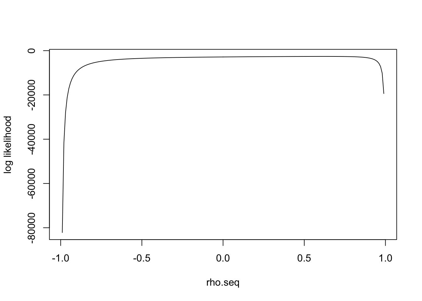
Expand here to see past versions of unnamed-chunk-15-1.png:
| Version | Author | Date |
|---|---|---|
| 568fbe6 | zouyuxin | 2018-08-13 |
\(l(\rho)'\) has one real solution
polyroot(c(- sum(data$Bhat[,1]*data$Bhat[,2]), - (n - sum(data$Bhat[,1]^2 + data$Bhat[,2]^2)), - sum(data$Bhat[,1]*data$Bhat[,2]), n))[1] 0.6193031+0.000000i 0.0058209+1.009339i 0.0058209-1.009339iIn general
The general derivation is in estimate correlation mle
Session information
sessionInfo()R version 3.5.1 (2018-07-02)
Platform: x86_64-apple-darwin15.6.0 (64-bit)
Running under: macOS High Sierra 10.13.6
Matrix products: default
BLAS: /Library/Frameworks/R.framework/Versions/3.5/Resources/lib/libRblas.0.dylib
LAPACK: /Library/Frameworks/R.framework/Versions/3.5/Resources/lib/libRlapack.dylib
locale:
[1] en_US.UTF-8/en_US.UTF-8/en_US.UTF-8/C/en_US.UTF-8/en_US.UTF-8
attached base packages:
[1] stats graphics grDevices utils datasets methods base
other attached packages:
[1] kableExtra_0.9.0 knitr_1.20 mashr_0.2-11 ashr_2.2-10
loaded via a namespace (and not attached):
[1] Rcpp_0.12.18 highr_0.7 pillar_1.3.0
[4] compiler_3.5.1 git2r_0.23.0 plyr_1.8.4
[7] workflowr_1.1.1 R.methodsS3_1.7.1 R.utils_2.6.0
[10] iterators_1.0.10 tools_3.5.1 digest_0.6.15
[13] viridisLite_0.3.0 tibble_1.4.2 evaluate_0.11
[16] lattice_0.20-35 pkgconfig_2.0.1 rlang_0.2.1
[19] Matrix_1.2-14 foreach_1.4.4 rstudioapi_0.7
[22] yaml_2.2.0 parallel_3.5.1 mvtnorm_1.0-8
[25] xml2_1.2.0 httr_1.3.1 stringr_1.3.1
[28] REBayes_1.3 hms_0.4.2 rprojroot_1.3-2
[31] grid_3.5.1 R6_2.2.2 rmarkdown_1.10
[34] rmeta_3.0 readr_1.1.1 magrittr_1.5
[37] whisker_0.3-2 scales_0.5.0 backports_1.1.2
[40] codetools_0.2-15 htmltools_0.3.6 MASS_7.3-50
[43] rvest_0.3.2 assertthat_0.2.0 colorspace_1.3-2
[46] stringi_1.2.4 Rmosek_8.0.69 munsell_0.5.0
[49] doParallel_1.0.11 pscl_1.5.2 truncnorm_1.0-8
[52] SQUAREM_2017.10-1 crayon_1.3.4 R.oo_1.22.0 This reproducible R Markdown analysis was created with workflowr 1.1.1