Estimate cor—max MASH
Yuxin Zou
2018-07-25
Last updated: 2018-08-15
library(mashr)Loading required package: ashrsource('../code/generateDataV.R')
source('../code/estimate_cor.R')
source('../code/summary.R')
library(knitr)
library(kableExtra)Apply the max methods for correlation matrix on mash data.
The estimated V from MLE(optim function) and EM perform better than the truncated correlation (error, mash log likelihood, ROC).
Comparing the estimated V from MLE and EM, EM algorithm tends to compute faster, and the estimated correlation is slightly better than the one from MLE in terms of estimation error, mash log likelihood, ROC.
One example
\[ \hat{\beta}|\beta \sim N_{3}(\hat{\beta}; \beta, \left(\begin{matrix} 1 & 0.7 & 0.2 \\ 0.7 & 1 & 0.4 \\ 0.2 & 0.4 & 1 \end{matrix}\right)) \]
\[ \beta \sim \frac{1}{4}\delta_{0} + \frac{1}{4}N_{3}(0, \left(\begin{matrix} 1 & 0 &0\\ 0 & 0 & 0 \\ 0 & 0 & 0 \end{matrix}\right)) + \frac{1}{4}N_{3}(0, \left(\begin{matrix} 1 & 0 & 0 \\ 0 & 1 & 0 \\ 0 & 0 & 0 \end{matrix}\right)) + \frac{1}{4}N_{3}(0, \left(\begin{matrix} 1 & 1 & 1 \\ 1 & 1 & 1 \\ 1 & 1 & 1 \end{matrix}\right)) \]
set.seed(1)
Sigma = cbind(c(1,0.7,0.2), c(0.7,1,0.4), c(0.2,0.4,1))
U0 = matrix(0,3,3)
U1 = matrix(0,3,3); U1[1,1] = 1
U2 = diag(3); U2[3,3] = 0
U3 = matrix(1,3,3)
data = generate_data(n=4000, p=3, V=Sigma, Utrue = list(U0=U0, U1=U1,U2=U2,U3=U3))
We find the estimate of V with canonical covariances and the PCA covariances.
m.data = mash_set_data(data$Bhat, data$Shat)
m.1by1 = mash_1by1(m.data)
strong = get_significant_results(m.1by1)

U.pca = cov_pca(m.data, 3, subset = strong)
U.ed = cov_ed(m.data, U.pca, subset = strong)
U.c = cov_canonical(m.data)
The PCA correlation matrices are: 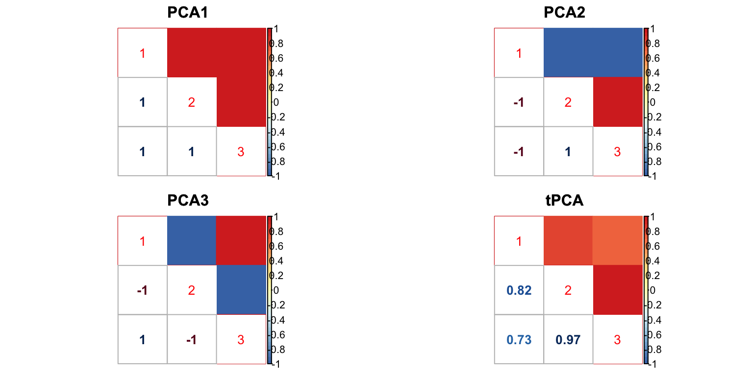
- We run the algorithm in estimate cor mle with 3 different initial points for \(\rho\) (-0.5,0,0.5). The \(\rho\) in each iteration is estimated using
optimfunction. The estimated correlation is
Vhat.mle = estimateV(m.data, c(U.c, U.ed), init_rho = c(-0.5,0,0.5), tol=1e-4, optmethod = 'mle')
Vhat.mle$V
[,1] [,2] [,3]
[1,] 1.0000000 0.7009268 0.1588733
[2,] 0.7009268 1.0000000 0.4001842
[3,] 0.1588733 0.4001842 1.0000000- The result uses algorithm in estimate cor em. \(\rho\) in each iteration is the root of a third degree polynomial.
Vhat.em = estimateV(m.data, c(U.c, U.ed), init_rho = c(-0.5,0,0.5), tol = 1e-4, optmethod = 'em2')
Vhat.em$V
[,1] [,2] [,3]
[1,] 1.0000000 0.7086927 0.1706391
[2,] 0.7086927 1.0000000 0.4187296
[3,] 0.1706391 0.4187296 1.0000000The running time (in sec.) for each pairwise correlation is
table = data.frame(rbind(Vhat.mle$ttime, Vhat.em$ttime), row.names = c('mle', 'em'))
colnames(table) = c('12','13','23')
table %>% kable() %>% kable_styling()| 12 | 13 | 23 | |
|---|---|---|---|
| mle | 290.737 | 207.046 | 68.977 |
| em | 168.826 | 63.495 | 51.343 |
The time is the total running time with different initial point.
- The result uses algorithm in estimate cor em V.
Vhat.emV = estimateV(m.data, c(U.c, U.ed), init_V = list(diag(ncol(m.data$Bhat)), clusterGeneration::rcorrmatrix(3), clusterGeneration::rcorrmatrix(3)), tol = 1e-4, optmethod = 'emV')
Vhat.emV$V
[,1] [,2] [,3]
[1,] 1.0000000 0.5487183 0.2669639
[2,] 0.5487183 1.0000000 0.4654711
[3,] 0.2669639 0.4654711 1.0000000- Using the original truncated correlation:
Vhat.tru = estimate_null_correlation(m.data)
Vhat.tru
[,1] [,2] [,3]
[1,] 1.0000000 0.4296283 0.1222433
[2,] 0.4296283 1.0000000 0.3324459
[3,] 0.1222433 0.3324459 1.0000000The truncated correlation underestimates the correlations.
- mash 1by1
V.mash = cor((data$Bhat/data$Shat)[-strong,])
V.mash
[,1] [,2] [,3]
[1,] 1.0000000 0.5313446 0.2445663
[2,] 0.5313446 1.0000000 0.4490049
[3,] 0.2445663 0.4490049 1.0000000Error
Check the estimation error:
FError = c(norm(Vhat.mle$V - Sigma, 'F'),
           norm(Vhat.em$V - Sigma, 'F'),
           norm(Vhat.emV$V - Sigma, 'F'),
           norm(Vhat.tru - Sigma, 'F'),
           norm(V.mash - Sigma, 'F'))
OpError = c(norm(Vhat.mle$V - Sigma, '2'),
           norm(Vhat.em$V - Sigma, '2'),
           norm(Vhat.emV$V - Sigma, '2'),
           norm(Vhat.tru - Sigma, '2'),
           norm(V.mash - Sigma, '2'))
table = data.frame(FrobeniusError = FError, SpectralError = OpError, row.names = c('mle','em','emV','trunc','m.1by1'))
table %>% kable() %>% kable_styling()| FrobeniusError | SpectralError | |
|---|---|---|
| mle | 0.0581773 | 0.0411417 |
| em | 0.0507627 | 0.0391489 |
| emV | 0.2516219 | 0.1960202 |
| trunc | 0.4091712 | 0.3049974 |
| m.1by1 | 0.2562509 | 0.1915171 |
mash log likelihood
In mash model, the model with correlation from mle has larger loglikelihood.
m.data.mle = mash_set_data(data$Bhat, data$Shat, V=Vhat.mle$V)
m.model.mle = mash(m.data.mle, c(U.c,U.ed), verbose = FALSE)
m.data.em = mash_set_data(data$Bhat, data$Shat, V=Vhat.em$V)
m.model.em = mash(m.data.em, c(U.c,U.ed), verbose = FALSE)m.data.emV = mash_set_data(data$Bhat, data$Shat, V=Vhat.emV$V)
m.model.emV = mash(m.data.emV, c(U.c,U.ed), verbose = FALSE)m.data.trunc = mash_set_data(data$Bhat, data$Shat, V=Vhat.tru)
m.model.trunc = mash(m.data.trunc, c(U.c,U.ed), verbose = FALSE)m.data.1by1 = mash_set_data(data$Bhat, data$Shat, V=V.mash)
m.model.1by1 = mash(m.data.1by1, c(U.c,U.ed), verbose = FALSE)m.data.correct = mash_set_data(data$Bhat, data$Shat, V=Sigma)
m.model.correct = mash(m.data.correct, c(U.c,U.ed), verbose = FALSE)The results are summarized in table:
null.ind = which(apply(data$B,1,sum) == 0)
V.trun = c(get_loglik(m.model.trunc), length(get_significant_results(m.model.trunc)), sum(get_significant_results(m.model.trunc) %in% null.ind))
V.mle = c(get_loglik(m.model.mle), length(get_significant_results(m.model.mle)), sum(get_significant_results(m.model.mle) %in% null.ind))
V.em = c(get_loglik(m.model.em), length(get_significant_results(m.model.em)), sum(get_significant_results(m.model.em) %in% null.ind))
V.emV = c(get_loglik(m.model.emV), length(get_significant_results(m.model.emV)), sum(get_significant_results(m.model.emV) %in% null.ind))
V.1by1 = c(get_loglik(m.model.1by1), length(get_significant_results(m.model.1by1)), sum(get_significant_results(m.model.1by1) %in% null.ind))
V.correct = c(get_loglik(m.model.correct), length(get_significant_results(m.model.correct)), sum(get_significant_results(m.model.correct) %in% null.ind))
temp = cbind(V.mle, V.em, V.emV, V.trun, V.1by1, V.correct)
colnames(temp) = c('MLE','EM','EMV', 'Truncate', 'm.1by1', 'True')
row.names(temp) = c('log likelihood', '# significance', '# False positive')
temp %>% kable() %>% kable_styling()| MLE | EM | EMV | Truncate | m.1by1 | True | |
|---|---|---|---|---|---|---|
| log likelihood | -17917.69 | -17919.23 | -17945.16 | -17951.46 | -17943.49 | -17913.58 |
| # significance | 146.00 | 149.00 | 82.00 | 85.00 | 73.00 | 149.00 |
| # False positive | 1.00 | 1.00 | 0.00 | 1.00 | 0.00 | 1.00 |
The estimated pi is
par(mfrow=c(2,3))
barplot(get_estimated_pi(m.model.mle), las=2, cex.names = 0.7, main='MLE', ylim=c(0,0.8))
barplot(get_estimated_pi(m.model.em), las=2, cex.names = 0.7, main='EM', ylim=c(0,0.8))
barplot(get_estimated_pi(m.model.emV), las=2, cex.names = 0.7, main='EMV', ylim=c(0,0.8))
barplot(get_estimated_pi(m.model.trunc), las=2, cex.names = 0.7, main='Truncate', ylim=c(0,0.8))
barplot(get_estimated_pi(m.model.1by1), las=2, cex.names = 0.7, main='m.1by1', ylim=c(0,0.8))
barplot(get_estimated_pi(m.model.correct), las=2, cex.names = 0.7, main='True', ylim=c(0,0.8))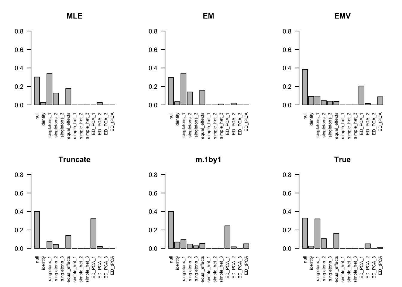
ROC
m.mle.seq = ROC.table(data$B, m.model.mle)
m.em.seq = ROC.table(data$B, m.model.em)
m.emV.seq = ROC.table(data$B, m.model.emV)
m.trun.seq = ROC.table(data$B, m.model.trunc)
m.1by1.seq = ROC.table(data$B, m.model.1by1)
m.correct.seq = ROC.table(data$B, m.model.correct)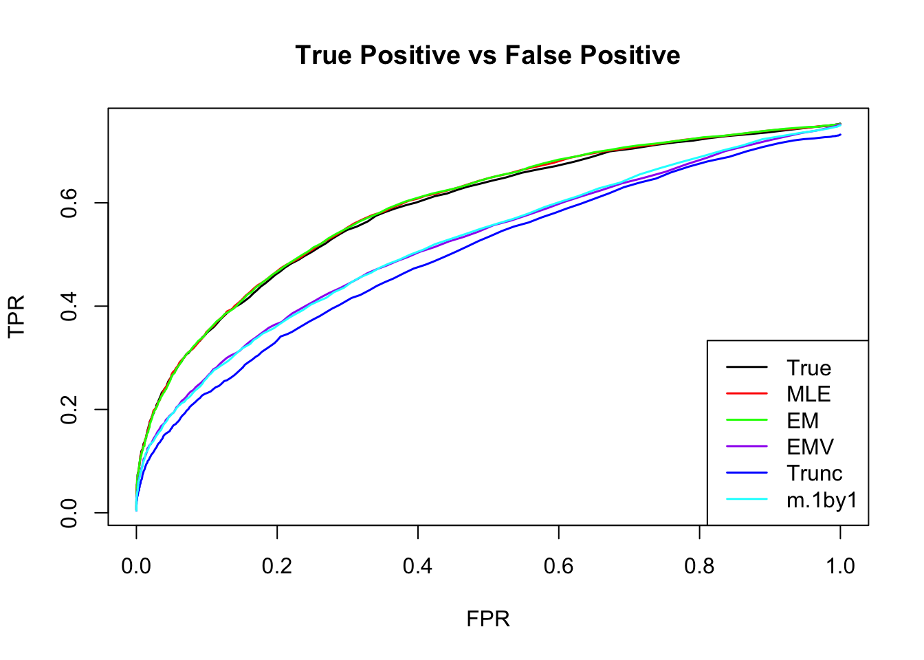
RRMSE
rrmse = rbind(RRMSE(data$B, data$Bhat, list(m.model.mle, m.model.em, m.model.emV, m.model.trunc, m.model.1by1, m.model.correct)))
colnames(rrmse) = c('MLE','EM','EMV', 'Truncate','m.1by1','True')
row.names(rrmse) = 'RRMSE'
rrmse %>% kable() %>% kable_styling()| MLE | EM | EMV | Truncate | m.1by1 | True | |
|---|---|---|---|---|---|---|
| RRMSE | 0.5277488 | 0.5285126 | 0.5437355 | 0.5592648 | 0.5442074 | 0.5283068 |
barplot(rrmse, ylim=c(0,(1+max(rrmse))/2), names.arg = c('MLE','EM', 'EMV','Truncate','m.1by1','True'), las=2, cex.names = 0.7, main='RRMSE')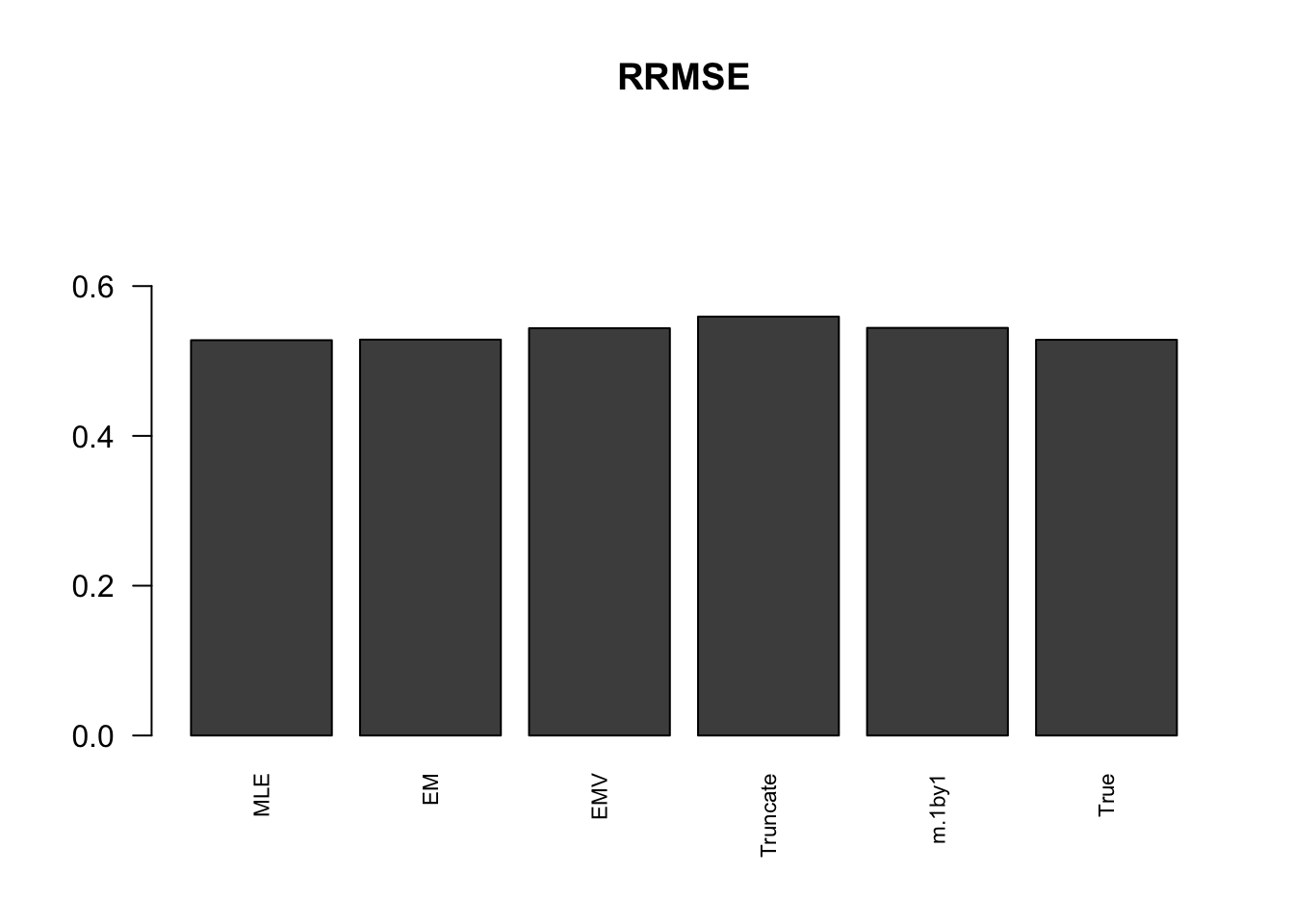
More simulations
I randomly generate 10 positive definite correlation matrices, V. The sample size is 4000.
\[ \hat{z}|z \sim N_{5}(z, V) \] \[ z\sim\frac{1}{4}\delta_{0} + \frac{1}{4}N_{5}(0,\left(\begin{matrix} 1 & \mathbf{0}_{1\times 4} \\ \mathbf{0}_{4\times 1} & \mathbf{0}_{4\times 4} \end{matrix}\right)) + \frac{1}{4}N_{5}(0,\left(\begin{matrix} \mathbf{1}_{2\times 2} & \mathbf{0}_{1\times 3} \\ \mathbf{0}_{3\times 1} & \mathbf{0}_{3\times 3} \end{matrix}\right)) + \frac{1}{4}N_{5}(0,\mathbf{1}_{5\times 5}) \]
set.seed(100)
n=4000; p = 5
U0 = matrix(0,p,p)
U1 = U0; U1[1,1] = 1
U2 = U0; U2[c(1:2), c(1:2)] = 1
U3 = matrix(1, p,p)
Utrue = list(U0 = U0, U1 = U1, U2 = U2, U3 = U3)
for(t in 1:10){
  Vtrue = clusterGeneration::rcorrmatrix(p)
  data = generate_data(n, p, Vtrue, Utrue)
  # mash cov
  m.data = mash_set_data(Bhat = data$Bhat, Shat = data$Shat)
  m.1by1 = mash_1by1(m.data)
  strong = get_significant_results(m.1by1)

  U.pca = cov_pca(m.data, 3, subset = strong)
  U.ed = cov_ed(m.data, U.pca, subset = strong)
  U.c = cov_canonical(m.data)
  Vhat.mle <- estimateV(m.data, c(U.c, U.ed), init_rho = c(-0.5,0,0.5), tol=1e-4, optmethod = 'mle')
  Vhat.em <- estimateV(m.data, c(U.c, U.ed), init_rho = c(-0.5,0,0.5), tol=1e-4, optmethod = 'em2')
  Vhat.emV <- estimateV(m.data, c(U.c, U.ed), init_V = list(diag(ncol(m.data$Bhat)), clusterGeneration::rcorrmatrix(p), clusterGeneration::rcorrmatrix(p)),tol=1e-4, optmethod = 'emV')
  saveRDS(list(V.true = Vtrue, V.mle = Vhat.mle, V.em = Vhat.em, V.emV = Vhat.emV, data = data, strong=strong),
          paste0('../output/MASH.result.',t,'.rds'))
}
files = dir("../output/AddEMV/"); files = files[grep("MASH.result",files)]
times = length(files)
result = vector(mode="list",length = times)
for(i in 1:times) {
result[[i]] = readRDS(paste("../output/AddEMV/", files[[i]], sep=""))
}mle.pd = numeric(times)
em.pd = numeric(times)
for(i in 1:times){
m.data = mash_set_data(result[[i]]$data$Bhat, result[[i]]$data$Shat)
result[[i]]$V.trun = estimate_null_correlation(m.data, apply_lower_bound = FALSE)
m.1by1 = mash_1by1(m.data)
strong = get_significant_results(m.1by1)
result[[i]]$V.1by1 = cor(m.data$Bhat[-strong,])
U.c = cov_canonical(m.data)
U.pca = cov_pca(m.data, 3, subset = strong)
U.ed = cov_ed(m.data, U.pca, subset = strong)
m.data.true = mash_set_data(Bhat = m.data$Bhat, Shat = m.data$Shat, V = result[[i]]$V.true)
m.model.true = mash(m.data.true, c(U.c,U.ed), verbose = FALSE)
m.data.trunc = mash_set_data(Bhat = m.data$Bhat, Shat = m.data$Shat, V = result[[i]]$V.trun)
m.model.trunc = mash(m.data.trunc, c(U.c,U.ed), verbose = FALSE)
m.data.1by1 = mash_set_data(Bhat = m.data$Bhat, Shat = m.data$Shat, V = result[[i]]$V.1by1)
m.model.1by1 = mash(m.data.1by1, c(U.c,U.ed), verbose = FALSE)
m.data.emV = mash_set_data(Bhat = m.data$Bhat, Shat = m.data$Shat, V = result[[i]]$V.emV$V)
m.model.emV = mash(m.data.emV, c(U.c,U.ed), verbose = FALSE)
# MLE
m.model.mle = m.model.mle.F = m.model.mle.2 = list()
R <- tryCatch(chol(result[[i]]$V.mle$V),error = function (e) FALSE)
if(is.matrix(R)){
mle.pd[i] = 1
m.data.mle = mash_set_data(Bhat = m.data$Bhat, Shat = m.data$Shat, V = result[[i]]$V.mle$V)
m.model.mle = mash(m.data.mle, c(U.c,U.ed), verbose = FALSE)
}else{
V.mle.near.F = as.matrix(Matrix::nearPD(result[[i]]$V.mle$V, conv.norm.type = 'F', keepDiag = TRUE)$mat)
V.mle.near.2 = as.matrix(Matrix::nearPD(result[[i]]$V.mle$V, conv.norm.type = '2', keepDiag = TRUE)$mat)
result[[i]]$V.mle.F = V.mle.near.F
result[[i]]$V.mle.2 = V.mle.near.2
# mashmodel
m.data.mle.F = mash_set_data(Bhat = m.data$Bhat, Shat = m.data$Shat, V = V.mle.near.F)
m.model.mle.F = mash(m.data.mle.F, c(U.c,U.ed), verbose = FALSE)
m.data.mle.2 = mash_set_data(Bhat = m.data$Bhat, Shat = m.data$Shat, V = V.mle.near.2)
m.model.mle.2 = mash(m.data.mle.2, c(U.c,U.ed), verbose = FALSE)
}
# EM
m.model.em = m.model.em.F = m.model.em.2 = list()
R <- tryCatch(chol(result[[i]]$V.em$V),error = function (e) FALSE)
if(is.matrix(R)){
em.pd[i] = 1
m.data.em = mash_set_data(Bhat = m.data$Bhat, Shat = m.data$Shat, V = result[[i]]$V.em$V)
m.model.em = mash(m.data.em, c(U.c,U.ed), verbose = FALSE)
}else{
V.em.near.F = as.matrix(Matrix::nearPD(result[[i]]$V.em$V, conv.norm.type = 'F', keepDiag = TRUE)$mat)
V.em.near.2 = as.matrix(Matrix::nearPD(result[[i]]$V.em$V, conv.norm.type = '2', keepDiag = TRUE)$mat)
result[[i]]$V.em.F = V.em.near.F
result[[i]]$V.em.2 = V.em.near.2
# mashmodel
m.data.em.F = mash_set_data(Bhat = m.data$Bhat, Shat = m.data$Shat, V = V.em.near.F)
m.model.em.F = mash(m.data.em.F, c(U.c,U.ed), verbose = FALSE)
m.data.em.2 = mash_set_data(Bhat = m.data$Bhat, Shat = m.data$Shat, V = V.em.near.2)
m.model.em.2 = mash(m.data.em.2, c(U.c,U.ed), verbose = FALSE)
}
result[[i]]$m.model = list(m.model.true = m.model.true, m.model.trunc = m.model.trunc,
m.model.1by1 = m.model.1by1, m.model.emV = m.model.emV,
m.model.mle = m.model.mle,
m.model.mle.F = m.model.mle.F, m.model.mle.2 = m.model.mle.2,
m.model.em = m.model.em,
m.model.em.F = m.model.em.F, m.model.em.2 = m.model.em.2)
}Error
Some estimated correlation matrices are not positive definite. So I estimate the nearest PD cor matrix with nearPD function.
The column with .F, .2 are from the nearest positive definite matrix with respect to Frobenius norm and spectral norm.
The Frobenius norm is
temp = matrix(0,nrow = times, ncol = 7)
for(i in 1:times){
  temp[i, ] = error.cor(result[[i]], norm.type='F', mle.pd = mle.pd[i], em.pd = em.pd[i])
}
colnames(temp) = c('Trunc','m.1by1', 'MLE','MLE.F', 'EM', 'EM.F', 'EMV')
temp[temp==0] = NA
temp %>% kable() %>% kable_styling()| Trunc | m.1by1 | MLE | MLE.F | EM | EM.F | EMV |
|---|---|---|---|---|---|---|
| 0.5847549 | 0.9286016 | 0.3185293 | 0.3053278 | 0.0941757 | NA | 1.0198618 |
| 0.6345196 | 0.8140108 | 0.1169154 | NA | 0.0981075 | NA | 0.8913631 |
| 0.7201453 | 0.9531300 | 0.2344733 | NA | 0.1734402 | NA | 1.0216638 |
| 0.8370832 | 1.0534335 | 0.1968091 | NA | 0.2411372 | NA | 1.1115619 |
| 0.8206008 | 0.8466408 | 0.1194142 | NA | 0.1189734 | NA | 0.9176794 |
| 0.8455747 | 1.1393764 | 0.1650726 | 0.1479670 | 0.1653665 | 0.1516188 | 1.2178752 |
| 0.5173056 | 0.8194980 | 0.1211599 | NA | 0.0861518 | NA | 0.8914736 |
| 0.8840057 | 0.9546138 | 0.1642744 | NA | 0.1563607 | NA | 1.0169747 |
| 0.6535878 | 1.0554833 | 0.1240352 | NA | 0.1323659 | NA | 1.1491978 |
| 0.6425639 | 0.9346341 | 0.0794776 | NA | 0.0700813 | NA | 1.0196620 |
The spectral norm is
temp = matrix(0,nrow = times, ncol = 7)
for(i in 1:times){
  temp[i, ] = error.cor(result[[i]], norm.type='2', mle.pd = mle.pd[i], em.pd = em.pd[i])
}
colnames(temp) = c('Trunc','m.1by1', 'MLE','MLE.2', 'EM', 'EM.2', 'EMV')
temp[temp==0] = NA
temp %>% kable() %>% kable_styling()| Trunc | m.1by1 | MLE | MLE.2 | EM | EM.2 | EMV |
|---|---|---|---|---|---|---|
| 0.4230698 | 0.7526315 | 0.2258153 | 0.2205340 | 0.0662442 | NA | 0.8335745 |
| 0.5228925 | 0.6281308 | 0.0783098 | NA | 0.0677285 | NA | 0.7069909 |
| 0.5156642 | 0.7945237 | 0.1750836 | NA | 0.1239438 | NA | 0.8577274 |
| 0.6529121 | 0.8335401 | 0.1484773 | NA | 0.1768351 | NA | 0.8944724 |
| 0.6500336 | 0.6377762 | 0.0778356 | NA | 0.0849870 | NA | 0.7052165 |
| 0.5607948 | 0.8613851 | 0.1001500 | 0.0937816 | 0.1085885 | 0.1015186 | 0.9343139 |
| 0.3157614 | 0.6406310 | 0.0795125 | NA | 0.0659174 | NA | 0.6982291 |
| 0.7134025 | 0.7290570 | 0.1090477 | NA | 0.1103719 | NA | 0.7987348 |
| 0.4767534 | 0.8894951 | 0.0964157 | NA | 0.0957622 | NA | 0.9760343 |
| 0.4591215 | 0.7926789 | 0.0568252 | NA | 0.0558999 | NA | 0.8740268 |
Time
The total running time for each matrix is
mle.time = em.time = numeric(times)
for(i in 1:times){
  mle.time[i] = sum(result[[i]]$V.mle$ttime)
  em.time[i] = sum(result[[i]]$V.em$ttime)
}
temp = cbind(mle.time, em.time)
colnames(temp) = c('MLE', 'EM')
row.names(temp) = 1:10
temp %>% kable() %>% kable_styling()| MLE | EM |
|---|---|
| 3171.983 | 848.351 |
| 2341.424 | 704.601 |
| 1990.764 | 740.046 |
| 3249.162 | 1072.233 |
| 1988.220 | 717.808 |
| 2580.794 | 958.710 |
| 1928.634 | 597.511 |
| 2992.277 | 1114.932 |
| 2339.513 | 708.779 |
| 2727.560 | 772.780 |
mash log likelihood
The NA means the estimated correlation matrix is not positive definite.
temp = matrix(0,nrow = times, ncol = 10)
for(i in 1:times){
  temp[i, ] = loglik.cor(result[[i]]$m.model, mle.pd = mle.pd[i], em.pd = em.pd[i])
}
colnames(temp) = c('True', 'Trunc','m.1by1', 'MLE','MLE.F', 'MLE.2', 'EM', 'EM.F', 'EM.2','EMV')
temp[temp == 0] = NA
temp[,-c(6,9)] %>% kable() %>% kable_styling()| True | Trunc | m.1by1 | MLE | MLE.F | EM | EM.F | EMV |
|---|---|---|---|---|---|---|---|
| -26039.92 | -26130.50 | -26112.94 | NA | -26265.49 | -26120.81 | NA | -26136.19 |
| -25669.59 | -26997.92 | -26950.67 | -26028.96 | NA | -25859.86 | NA | -26967.47 |
| -27473.71 | -27547.11 | -27535.67 | -27465.76 | NA | -27463.43 | NA | -27551.75 |
| -28215.48 | -28604.98 | -28646.72 | -28301.41 | NA | -28338.57 | NA | -28669.24 |
| -24988.68 | -25236.18 | -25110.41 | -25056.59 | NA | -25048.86 | NA | -25123.96 |
| -24299.89 | -24978.79 | -24972.25 | NA | -24492.32 | NA | -24478.09 | -25020.38 |
| -27574.71 | -27698.40 | -27662.48 | -27517.65 | NA | -27540.65 | NA | -27684.83 |
| -27941.86 | -28159.65 | -28182.04 | -27979.99 | NA | -27953.02 | NA | -28222.45 |
| -29788.75 | -29824.45 | -29921.87 | -29760.81 | NA | -29759.50 | NA | -29954.96 |
| -28542.34 | -28922.58 | -29163.51 | -28537.96 | NA | -28550.73 | NA | -29221.61 |
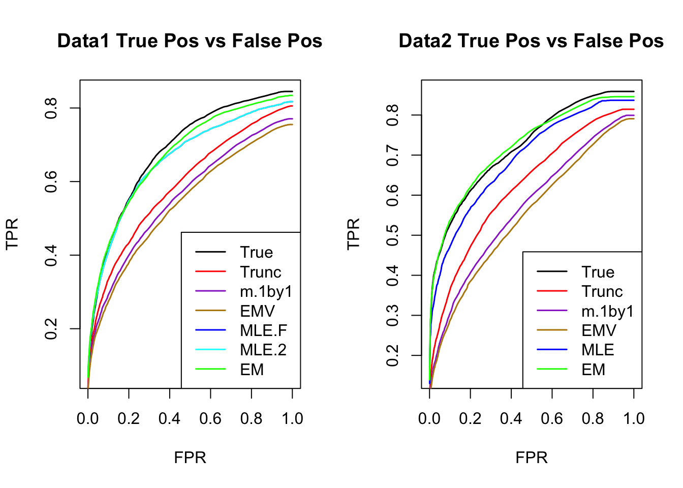
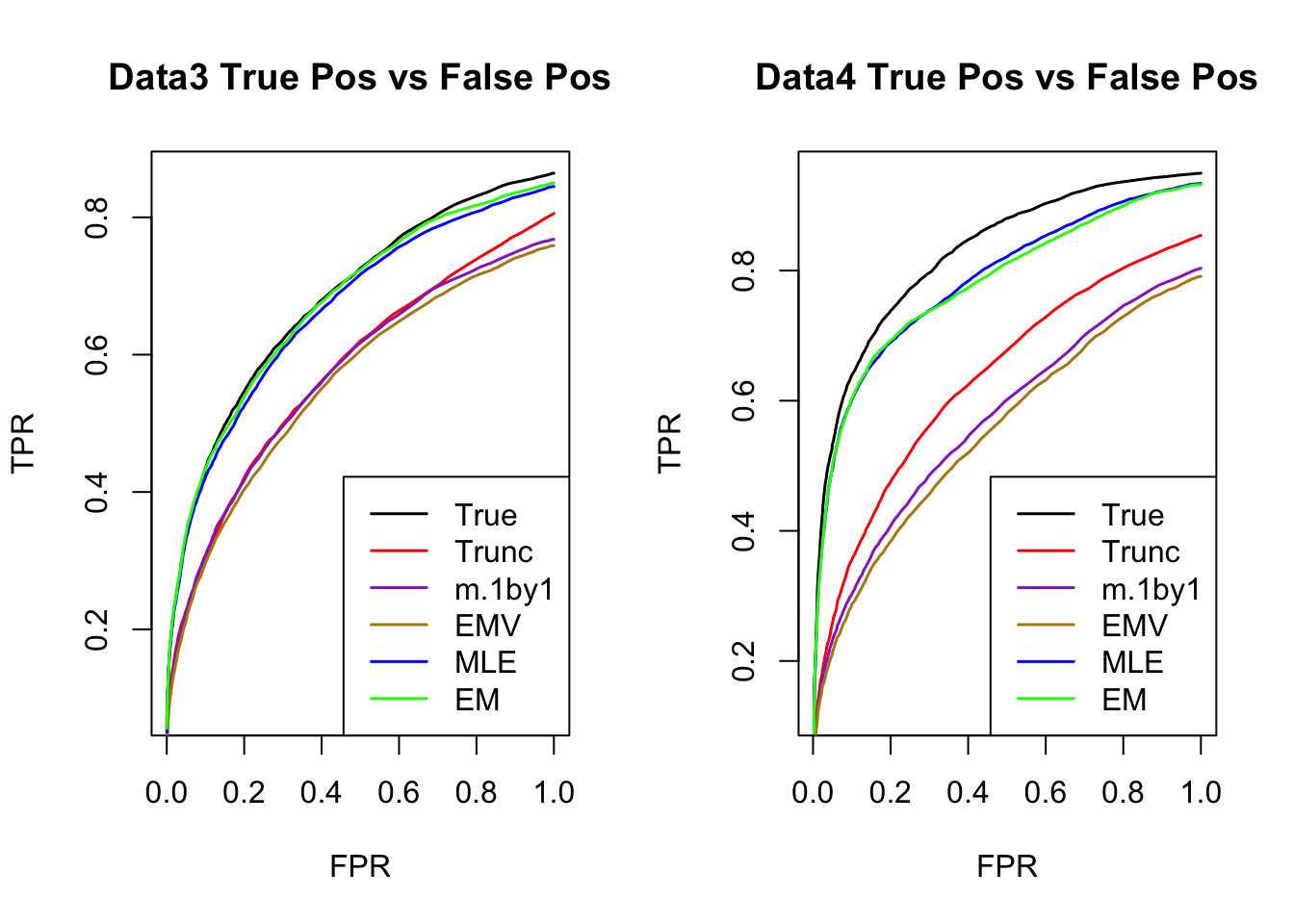
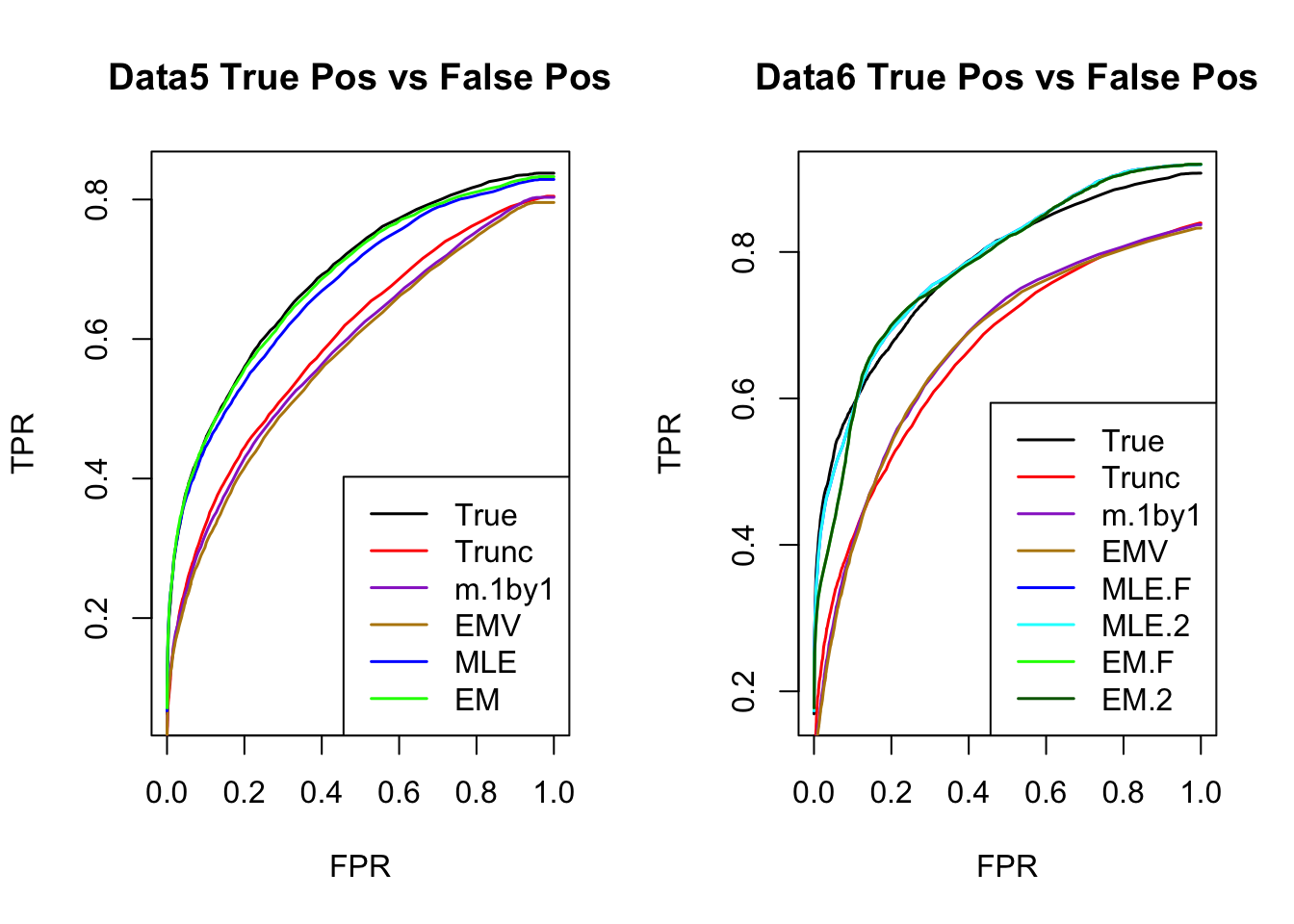
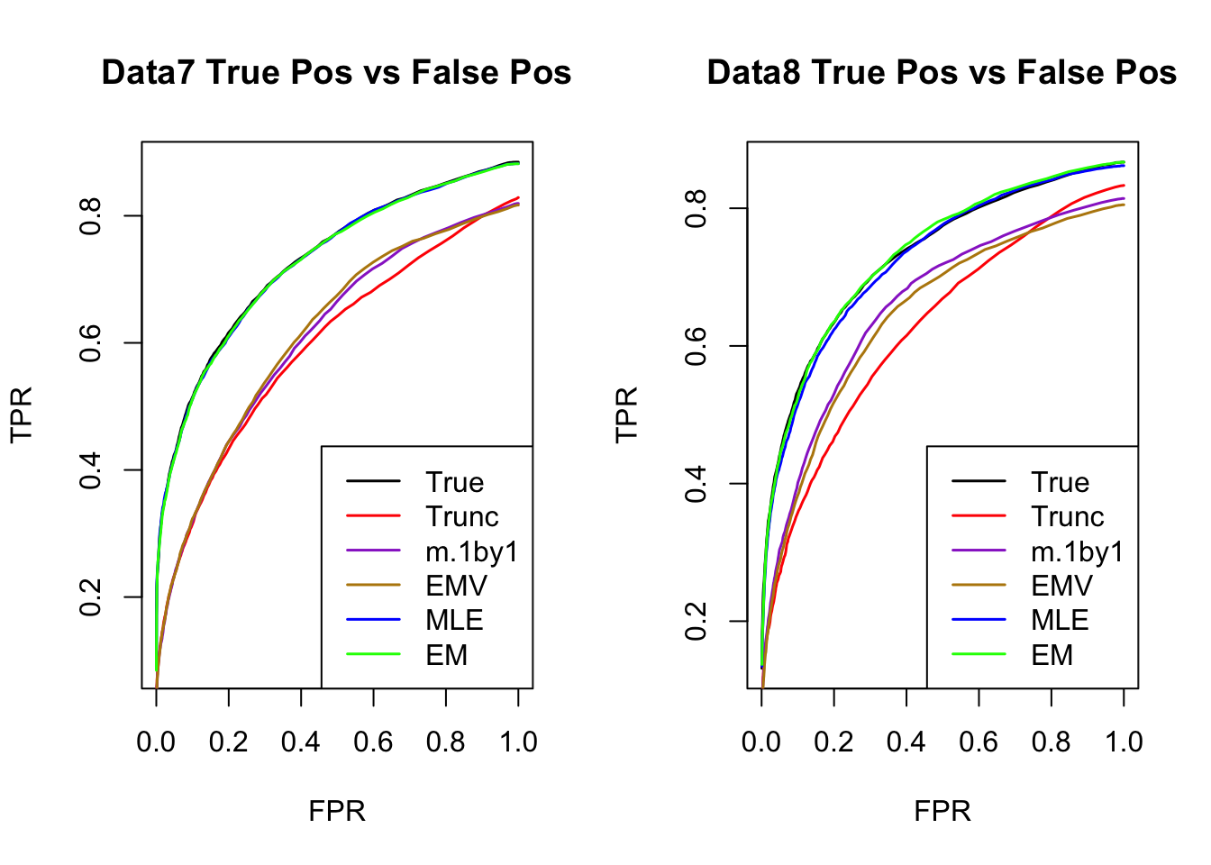
ROC
par(mfrow=c(1,2))
for(i in 1:times){
  plotROC(result[[i]]$data$B, result[[i]]$m.model, mle.pd = mle.pd[i], em.pd = em.pd[i], title=paste0('Data', i, ' '))
}

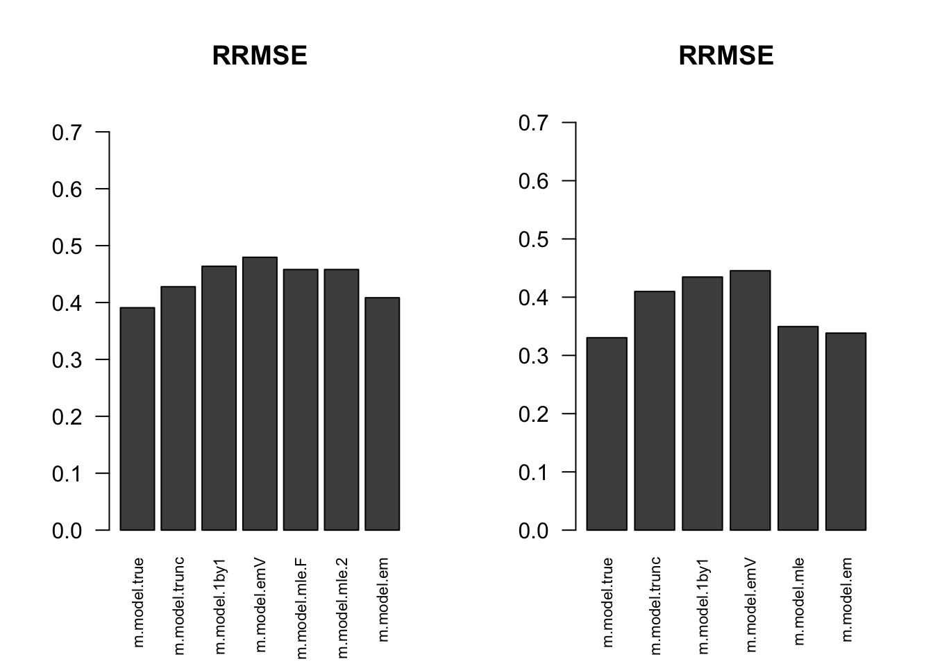
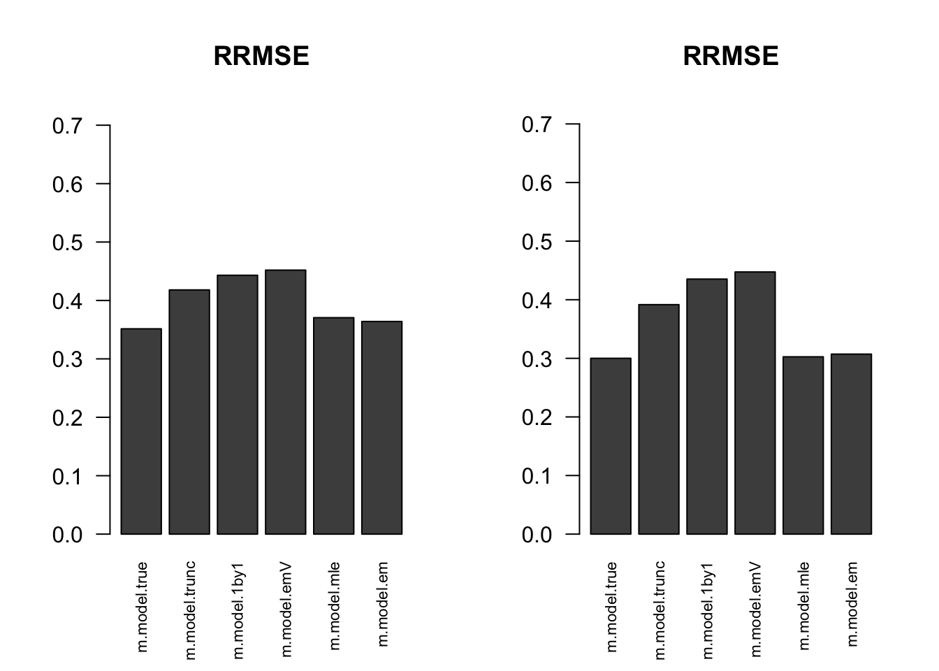
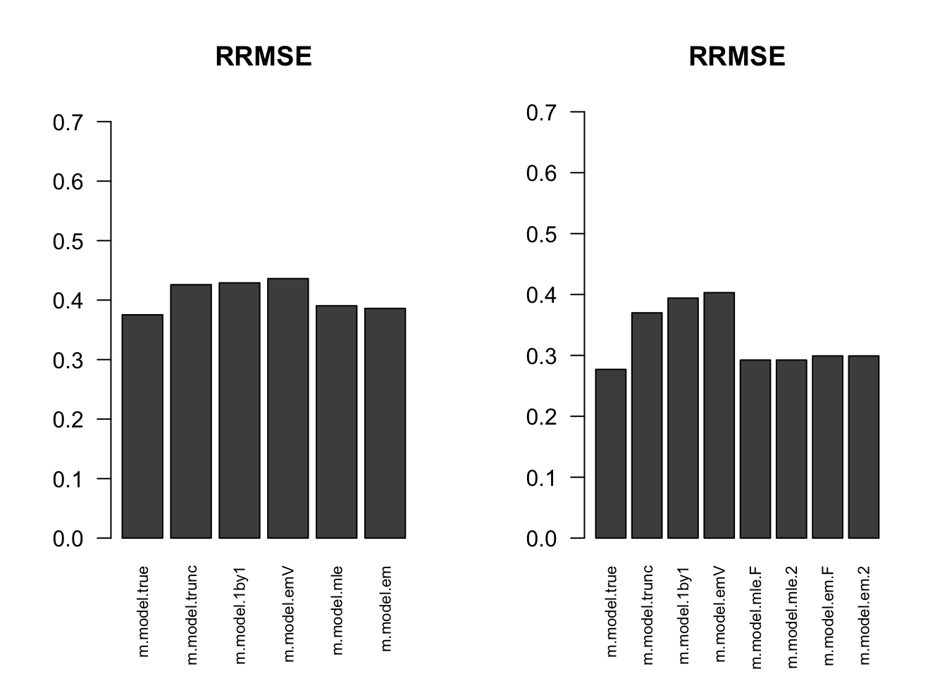
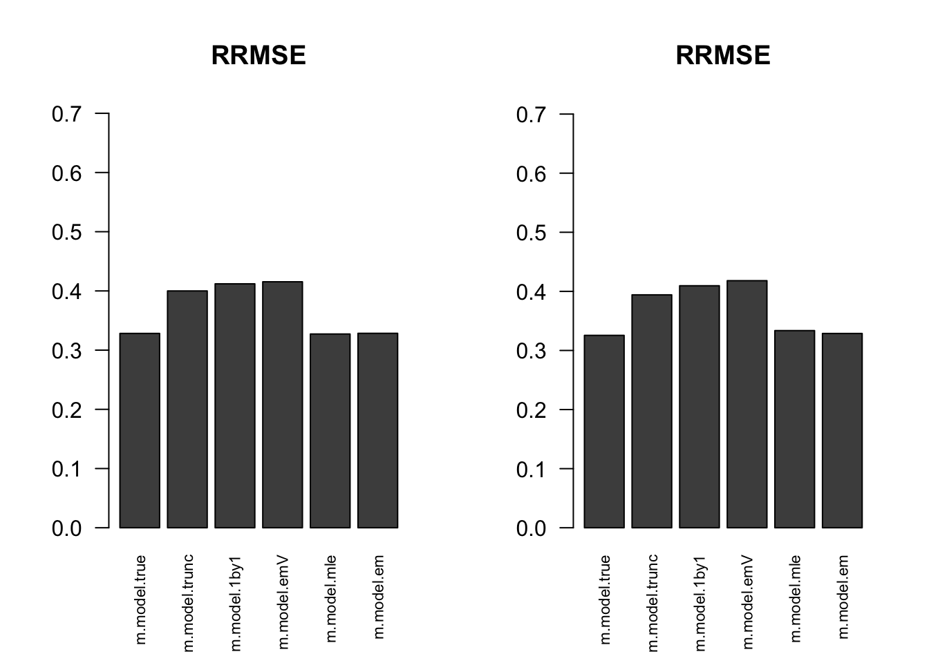
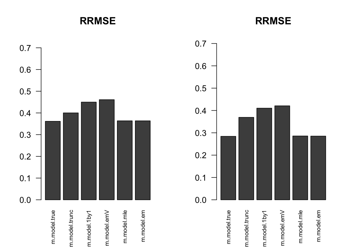
RRMSE
par(mfrow=c(1,2))
for(i in 1:times){
  rrmse = rbind(RRMSE(result[[i]]$data$B, result[[i]]$data$Bhat, result[[i]]$m.model))
  barplot(rrmse, ylim=c(0,(1+max(rrmse))/2), las=2, cex.names = 0.7, main='RRMSE')
}
Session information
sessionInfo()R version 3.5.1 (2018-07-02)
Platform: x86_64-apple-darwin15.6.0 (64-bit)
Running under: macOS High Sierra 10.13.6
Matrix products: default
BLAS: /Library/Frameworks/R.framework/Versions/3.5/Resources/lib/libRblas.0.dylib
LAPACK: /Library/Frameworks/R.framework/Versions/3.5/Resources/lib/libRlapack.dylib
locale:
[1] en_US.UTF-8/en_US.UTF-8/en_US.UTF-8/C/en_US.UTF-8/en_US.UTF-8
attached base packages:
[1] stats graphics grDevices utils datasets methods base
other attached packages:
[1] kableExtra_0.9.0 knitr_1.20 mashr_0.2-11 ashr_2.2-10
loaded via a namespace (and not attached):
[1] Rcpp_0.12.18 highr_0.7
[3] compiler_3.5.1 pillar_1.3.0
[5] plyr_1.8.4 iterators_1.0.10
[7] tools_3.5.1 corrplot_0.84
[9] digest_0.6.15 viridisLite_0.3.0
[11] evaluate_0.11 tibble_1.4.2
[13] lattice_0.20-35 pkgconfig_2.0.1
[15] rlang_0.2.1 Matrix_1.2-14
[17] foreach_1.4.4 rstudioapi_0.7
[19] yaml_2.2.0 parallel_3.5.1
[21] mvtnorm_1.0-8 xml2_1.2.0
[23] httr_1.3.1 stringr_1.3.1
[25] REBayes_1.3 hms_0.4.2
[27] rprojroot_1.3-2 grid_3.5.1
[29] R6_2.2.2 rmarkdown_1.10
[31] rmeta_3.0 readr_1.1.1
[33] magrittr_1.5 scales_0.5.0
[35] backports_1.1.2 codetools_0.2-15
[37] htmltools_0.3.6 MASS_7.3-50
[39] rvest_0.3.2 assertthat_0.2.0
[41] colorspace_1.3-2 stringi_1.2.4
[43] Rmosek_8.0.69 munsell_0.5.0
[45] pscl_1.5.2 doParallel_1.0.11
[47] truncnorm_1.0-8 SQUAREM_2017.10-1
[49] clusterGeneration_1.3.4 ExtremeDeconvolution_1.3
[51] crayon_1.3.4 This R Markdown site was created with workflowr