SuSiE Z Problem
Yuxin Zou
1/17/2019
Last updated: 2019-01-17
workflowr checks: (Click a bullet for more information)-
✔ R Markdown file: up-to-date
Great! Since the R Markdown file has been committed to the Git repository, you know the exact version of the code that produced these results.
-
✔ Environment: empty
Great job! The global environment was empty. Objects defined in the global environment can affect the analysis in your R Markdown file in unknown ways. For reproduciblity it’s best to always run the code in an empty environment.
-
✔ Seed:
set.seed(20190115)The command
set.seed(20190115)was run prior to running the code in the R Markdown file. Setting a seed ensures that any results that rely on randomness, e.g. subsampling or permutations, are reproducible. -
✔ Session information: recorded
Great job! Recording the operating system, R version, and package versions is critical for reproducibility.
-
Great! You are using Git for version control. Tracking code development and connecting the code version to the results is critical for reproducibility. The version displayed above was the version of the Git repository at the time these results were generated.✔ Repository version: fd55060
Note that you need to be careful to ensure that all relevant files for the analysis have been committed to Git prior to generating the results (you can usewflow_publishorwflow_git_commit). workflowr only checks the R Markdown file, but you know if there are other scripts or data files that it depends on. Below is the status of the Git repository when the results were generated:
Note that any generated files, e.g. HTML, png, CSS, etc., are not included in this status report because it is ok for generated content to have uncommitted changes.Ignored files: Ignored: .Rhistory Ignored: .Rproj.user/ Ignored: .sos/ Ignored: data/.DS_Store Untracked files: Untracked: .gitattributes Untracked: analysis/SusieZConverge.Rmd Untracked: data/sim_gaussian_475.rds Untracked: data/sim_gaussian_75.rds Untracked: output/dscout_gaussian_init.rds Untracked: output/dscout_gaussian_null.rds Untracked: output/dscout_gaussian_z.rds Unstaged changes: Modified: analysis/dscquery.Rmd
Expand here to see past versions:
Investigate the non-convergence problem in susie_z.
devtools::install_github('zouyuxin/susieR')Skipping install of 'susieR' from a github remote, the SHA1 (7cd1fa2d) has not changed since last install.
Use `force = TRUE` to force installationlibrary(susieR)Simulation under null effect
dscout_null = readRDS('output/dscout_gaussian_null.rds')
dscout_null = dscout_null[!is.na(dscout_null$sim_gaussian_null.output.file),]
dscout_null = dscout_null[!is.na(dscout_null$susie_z.output.file),]
The maximum number of iteration is 7. All models converge. There is no false discovry.
Simulation with one effect
We simulate data with only one non-zero effect.
We simulate data under PVE = 0.01, 0.05, 0.1, 0.2, 0.5, 0.8, 0.95. There are 20 replicates.
dscout_gaussian_z = readRDS('output/dscout_gaussian_z.rds')
dscout_gaussian_z = dscout_gaussian_z[!is.na(dscout_gaussian_z$sim_gaussian.output.file),]
dscout_gaussian_z = dscout_gaussian_z[!is.na(dscout_gaussian_z$susie_z.output.file),]
dscout_gaussian_z$NotConverge = dscout_gaussian_z$susie_z.niter == 100
dscout_gaussian_z_1 = dscout_gaussian_z[dscout_gaussian_z$sim_gaussian.effect_num == '1', ]
dscout_gaussian_z_1 = dscout_gaussian_z_1[dscout_gaussian_z_1$susie_z.L == '5' , ]When the PVE is greater than 0.5, some replicates fail to converge in 100 iterations.
converge.summary = aggregate(NotConverge ~ sim_gaussian.pve, dscout_gaussian_z_1, sum)
colnames(converge.summary) = c('pve', 'NotConverge')
converge.summary
pve NotConverge
1 0.01 0
2 0.05 0
3 0.10 0
4 0.20 0
5 0.50 4
6 0.80 9
7 0.95 6Now we change the initial susie object to the truth:
dscout_gaussian_init = readRDS('output/dscout_gaussian_init.rds')
dscout_gaussian_init = dscout_gaussian_init[!is.na(dscout_gaussian_init$sim_gaussian.output.file),]
dscout_gaussian_init = dscout_gaussian_init[!is.na(dscout_gaussian_init$susie_z_init.output.file),]
dscout_gaussian_init$NotConverge = dscout_gaussian_init$susie_z_init.niter == 100
dscout_gaussian_init_1 = dscout_gaussian_init[dscout_gaussian_init$sim_gaussian.effect_num == '1', ]converge.summary = aggregate(NotConverge ~ sim_gaussian.pve, dscout_gaussian_init_1, sum)
colnames(converge.summary) = c('pve', 'NotConverge')
converge.summary pve NotConverge
1 0.01 0
2 0.05 0
3 0.10 0
4 0.20 0
5 0.50 0
6 0.80 0
7 0.95 0All models converge.
Simulation with 5 effects
We simulate data with 5 true effects. We simulate data under PVE = 0.01, 0.05, 0.1, 0.2, 0.5, 0.8, 0.95. There are 20 replicates.
dscout_gaussian_z_5 = dscout_gaussian_z[dscout_gaussian_z$sim_gaussian.effect_num == '5', ]
dscout_gaussian_z_5 = dscout_gaussian_z_5[dscout_gaussian_z_5$susie_z.L == '5' , ]
When the PVE is greater than 0.5, some replicates fail to converge in 100 iterations.
converge.summary = aggregate(NotConverge ~ sim_gaussian.pve, dscout_gaussian_z_5, sum)
colnames(converge.summary) = c('pve', 'NotConverge')
converge.summary
pve NotConverge
1 0.01 0
2 0.05 0
3 0.10 0
4 0.20 0
5 0.50 1
6 0.80 5
7 0.95 5Now we change the initial susie object to the truth,
dscout_gaussian_init_5 = dscout_gaussian_init[dscout_gaussian_init$sim_gaussian.effect_num == '5', ]converge.summary = aggregate(NotConverge ~ sim_gaussian.pve, dscout_gaussian_init_5, sum)
colnames(converge.summary) = c('pve', 'NotConverge')
converge.summary pve NotConverge
1 0.01 0
2 0.05 0
3 0.10 0
4 0.20 0
5 0.50 1
6 0.80 5
7 0.95 5There are still non-convergence cases with the true initialization.
Examples
One effect
Let’s see an example data with one true effect. The PVE is 0.5, the residual variance is 0.47^2.
X = readRDS('data/susie_X.rds') # X is from susieR package, N3finemapping, X is coloumn mean centered.
R = readRDS('data/susie_R.rds')
data = readRDS('data/sim_gaussian_75.rds')
n = data$n
beta = numeric(data$p)
beta[data$beta_idx] = data$beta_val
z = data$ss$effect/data$ss$se
susie_plot(z, y = 'z', b=beta)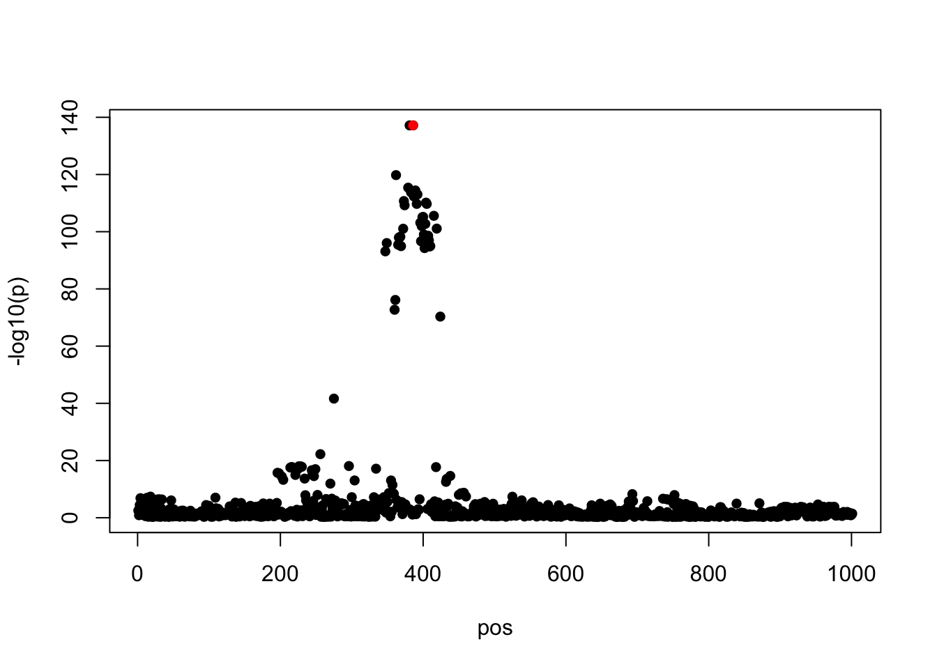
Expand here to see past versions of unnamed-chunk-13-1.png:
| Version | Author | Date |
|---|---|---|
| a6cee3a | zouyuxin | 2019-01-17 |
Using z scores,
fit_z = susie_z(z, R=R, max_iter = 20, L=5, track_fit = T)Warning in susie_ss(XtX = R, Xty = z, n = 2, var_y = 1, L = L,
estimate_prior_variance = TRUE, : IBSS algorithm did not converge in 20
iterations!susie_get_objective(fit_z)[1] 409.0831susie_plot(fit_z, y = 'PIP', b = beta)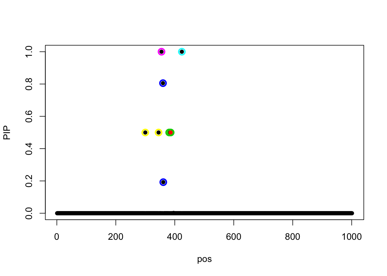
Expand here to see past versions of unnamed-chunk-14-1.png:
| Version | Author | Date |
|---|---|---|
| a6cee3a | zouyuxin | 2019-01-17 |
Now we initialize at the truth (L=1), the model converges to a lower objective value.
s_init = susie_init_coef(data$beta_idx, data$beta_val, data$p)
fit_z_init = susie_z(z, R=R, s_init = s_init)
susie_get_objective(fit_z_init)
[1] 299.4515susie_plot(fit_z_init, y = 'PIP', b = beta)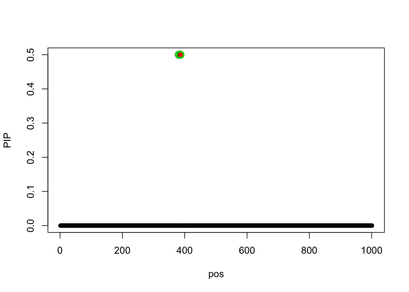
Expand here to see past versions of unnamed-chunk-15-1.png:
| Version | Author | Date |
|---|---|---|
| a6cee3a | zouyuxin | 2019-01-17 |
I mentioned in the write-up, we approximate the BF(\(z_j(\sigma)\)) (eqn 7.61) using BF(\(z_j(\hat{\sigma}_j)\)). When the data contain strong association signals (\(\hat{\sigma}_j > \sigma\)), the z score approximation under-estimates the Bayes Factor.
The 7.61 in the write-up: \[ \begin{align} BF(z_j(\sigma); w) &= \sqrt{\frac{1}{1+w^2}} \exp\left( \frac{1}{2} z_j(\sigma)^2 \frac{w^2}{1+w^2} \right) \quad \quad \text{where }w^2 = (n-1)\frac{\sigma_{0}^{2}}{\sigma^2} \end{align} \]
We check the under-estimate now:
fit_z_1 = susie_ss(XtX = R, Xty = z, n = 2, var_y = 1, L = 1,
                   estimate_prior_variance = FALSE,
                   estimate_residual_variance = FALSE, max_iter = 1)
X.s = apply(X, 2, function(x) x/(sd(x)*sqrt(n-1)))
z_true = (t(X.s) %*% data$sim_y) / as.numeric(data$sigma)
fit_z_1_true = susie_ss(XtX = R, Xty = z_true, n = 2, var_y = 1, L = 1,
estimate_prior_variance = FALSE,
estimate_residual_variance = FALSE,
prior_weights = NULL, null_weight = NULL,
coverage = 0.95, min_abs_corr = 0.5,
verbose = FALSE, track_fit = TRUE, max_iter = 1)par(mfrow=c(1,3))
{plot(fit_z_1$lbf_mtx, fit_z_1_true$lbf_mtx, xlab = expression(logBF(z[j](hat(sigma)[j]))), ylab = expression(logBF(z[j](sigma))), main='log BF')
abline(0,1)}
{plot(fit_z_1$alpha, fit_z_1_true$alpha, xlab = expression(alpha(hat(sigma)[j])), ylab = expression(alpha(sigma)), main=expression(alpha))
abline(0,1)}
{plot(abs(fit_z_1$mu), abs(fit_z_1_true$mu), xlab = expression(abs(mu(hat(sigma)[j]))), ylab = expression(abs(mu(sigma))), main=expression(abs(mu)))
abline(0,1)}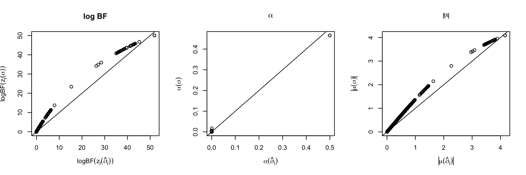
Expand here to see past versions of unnamed-chunk-18-1.png:
| Version | Author | Date |
|---|---|---|
| a6cee3a | zouyuxin | 2019-01-17 |
It is clear from the plot that the Bayes Factor is under-estimated. The estimated \(\alpha\), \(\mu\) are smaller.
Checked the estimated prior variance,
fit_z_10_prior = susie_z(z=z, R=R, L=5)Warning in susie_ss(XtX = R, Xty = z, n = 2, var_y = 1, L = L,
estimate_prior_variance = TRUE, : IBSS algorithm did not converge in 100
iterations!susie_get_prior_variance(fit_z_10_prior)[1] 24449.0562 4961.9053 2624.2558 2017.4113 163.6263fit_z_10_true_prior = susie_z(z = z_true, R=R, L=5)
susie_get_prior_variance(fit_z_10_true_prior)[1] 604.074353 3.315658 0.000000 0.000000 0.000000susie_plot(fit_z_10_true_prior, y='PIP', b=beta)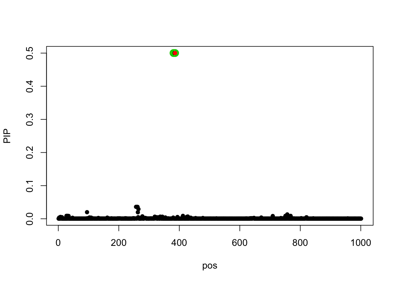
Expand here to see past versions of unnamed-chunk-20-1.png:
| Version | Author | Date |
|---|---|---|
| a6cee3a | zouyuxin | 2019-01-17 |
Using the true z, \(z_j(\sigma)\), the estimated prior variance for some L becomes zero. Using the estimated z, \(z_j(\hat{\sigma}_j)\), the estimated prior variance for all L are non-zero.
Five effects
Let’s see an example data with 5 true effects. The PVE is 0.8, the residual variance is 0.74^2.
data = readRDS('data/sim_gaussian_475.rds')
n = data$n
beta = numeric(data$p)
beta[data$beta_idx] = data$beta_val
z = data$ss$effect/data$ss$se
susie_plot(z, y = "z", b=beta)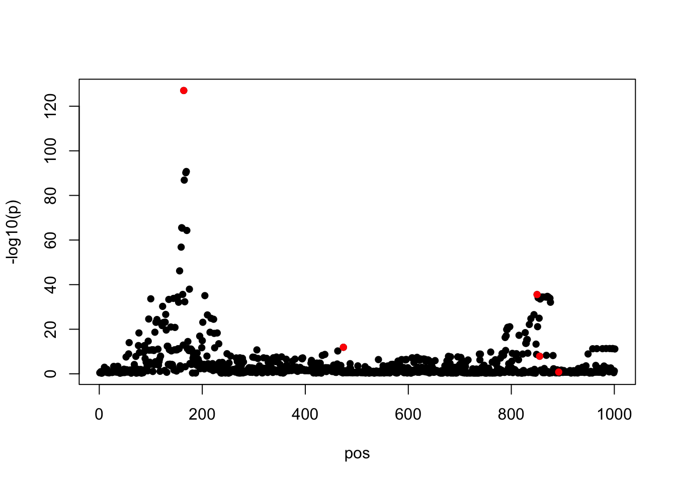
Expand here to see past versions of unnamed-chunk-21-1.png:
| Version | Author | Date |
|---|---|---|
| a6cee3a | zouyuxin | 2019-01-17 |
Using z scores,
fit_z = susie_z(z, R=R, max_iter = 20, L=5, track_fit = T)Warning in susie_ss(XtX = R, Xty = z, n = 2, var_y = 1, L = L,
estimate_prior_variance = TRUE, : IBSS algorithm did not converge in 20
iterations!susie_get_objective(fit_z)[1] 525.9303susie_plot(fit_z, y = 'PIP', b = beta)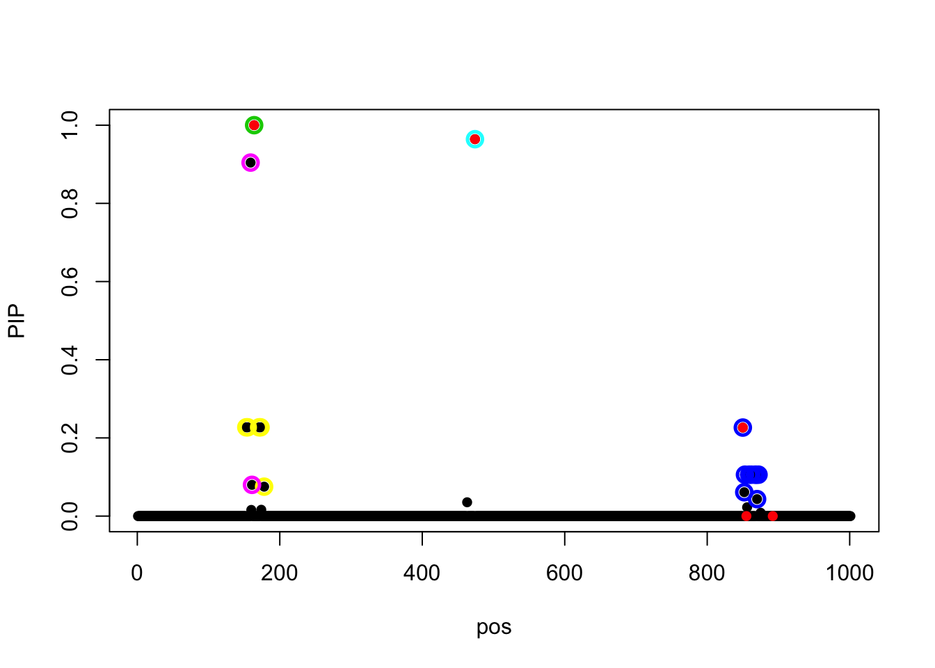
Expand here to see past versions of unnamed-chunk-22-1.png:
| Version | Author | Date |
|---|---|---|
| a6cee3a | zouyuxin | 2019-01-17 |
Now we initialize at the truth, the model fails to converge.
s_init = susie_init_coef(data$beta_idx, data$beta_val, data$p)
fit_z_init = susie_z(z, R=R, s_init = s_init)
Warning in susie_ss(XtX = R, Xty = z, n = 2, var_y = 1, L = L,
estimate_prior_variance = TRUE, : IBSS algorithm did not converge in 100
iterations!susie_get_objective(fit_z_init)[1] 1089.854susie_plot(fit_z_init, y = 'PIP', b = beta)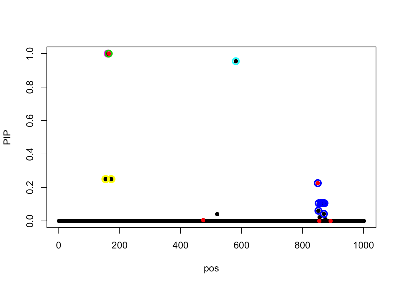
Expand here to see past versions of unnamed-chunk-23-1.png:
| Version | Author | Date |
|---|---|---|
| a6cee3a | zouyuxin | 2019-01-17 |
Changing the z score to \(z_j(\sigma)\), the model converges.
z_true = (t(X.s) %*% data$sim_y) / as.numeric(data$sigma)
fit_z_5_true = susie_z(z = z_true, R=R, L=5)
susie_get_objective(fit_z_5_true)
[1] 1119.521susie_get_prior_variance(fit_z_5_true)[1] 1467.02402 640.34084 185.85349 53.12493 0.00000susie_plot(fit_z_5_true, y = 'PIP', b = beta)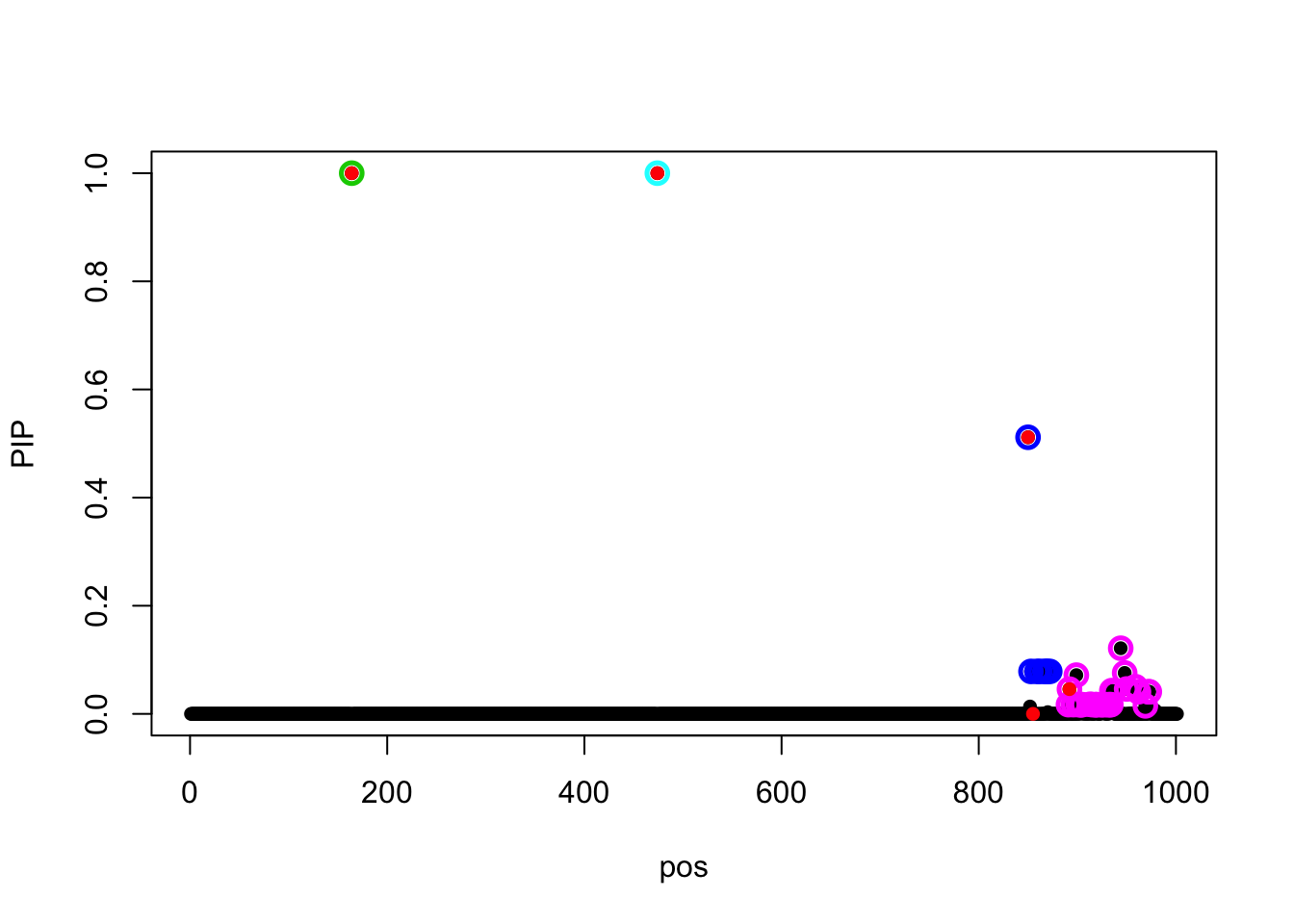
Expand here to see past versions of unnamed-chunk-24-1.png:
| Version | Author | Date |
|---|---|---|
| a6cee3a | zouyuxin | 2019-01-17 |
Session information
sessionInfo()R version 3.5.1 (2018-07-02)
Platform: x86_64-apple-darwin15.6.0 (64-bit)
Running under: macOS 10.14.2
Matrix products: default
BLAS: /Library/Frameworks/R.framework/Versions/3.5/Resources/lib/libRblas.0.dylib
LAPACK: /Library/Frameworks/R.framework/Versions/3.5/Resources/lib/libRlapack.dylib
locale:
[1] en_US.UTF-8/en_US.UTF-8/en_US.UTF-8/C/en_US.UTF-8/en_US.UTF-8
attached base packages:
[1] stats graphics grDevices utils datasets methods base
other attached packages:
[1] susieR_0.6.3
loaded via a namespace (and not attached):
[1] Rcpp_1.0.0 compiler_3.5.1 git2r_0.24.0
[4] workflowr_1.1.1 R.methodsS3_1.7.1 prettyunits_1.0.2
[7] R.utils_2.7.0 remotes_2.0.2 tools_3.5.1
[10] testthat_2.0.1 digest_0.6.18 pkgbuild_1.0.2
[13] pkgload_1.0.2 lattice_0.20-38 evaluate_0.12
[16] memoise_1.1.0 rlang_0.3.1 Matrix_1.2-15
[19] cli_1.0.1 curl_3.3 yaml_2.2.0
[22] expm_0.999-3 withr_2.1.2 stringr_1.3.1
[25] knitr_1.20 desc_1.2.0 fs_1.2.6
[28] devtools_2.0.1 grid_3.5.1 rprojroot_1.3-2
[31] glue_1.3.0 R6_2.3.0 processx_3.2.1
[34] rmarkdown_1.11 sessioninfo_1.1.1 callr_3.1.1
[37] magrittr_1.5 whisker_0.3-2 backports_1.1.3
[40] ps_1.3.0 htmltools_0.3.6 usethis_1.4.0
[43] assertthat_0.2.0 stringi_1.2.4 crayon_1.3.4
[46] R.oo_1.22.0 This reproducible R Markdown analysis was created with workflowr 1.1.1