Gaussian variance estimation in simulated data sets
Zhengrong Xing, Peter Carbonetto and Matthew Stephens
Last updated: 2018-11-09
workflowr checks: (Click a bullet for more information)-
✔ R Markdown file: up-to-date
Great! Since the R Markdown file has been committed to the Git repository, you know the exact version of the code that produced these results.
-
✔ Environment: empty
Great job! The global environment was empty. Objects defined in the global environment can affect the analysis in your R Markdown file in unknown ways. For reproduciblity it’s best to always run the code in an empty environment.
-
✔ Seed:
set.seed(1)The command
set.seed(1)was run prior to running the code in the R Markdown file. Setting a seed ensures that any results that rely on randomness, e.g. subsampling or permutations, are reproducible. -
✔ Session information: recorded
Great job! Recording the operating system, R version, and package versions is critical for reproducibility.
-
Great! You are using Git for version control. Tracking code development and connecting the code version to the results is critical for reproducibility. The version displayed above was the version of the Git repository at the time these results were generated.✔ Repository version: 8214f9d
Note that you need to be careful to ensure that all relevant files for the analysis have been committed to Git prior to generating the results (you can usewflow_publishorwflow_git_commit). workflowr only checks the R Markdown file, but you know if there are other scripts or data files that it depends on. Below is the status of the Git repository when the results were generated:
Note that any generated files, e.g. HTML, png, CSS, etc., are not included in this status report because it is ok for generated content to have uncommitted changes.Ignored files: Ignored: dsc/code/Wavelab850/MEXSource/CPAnalysis.mexmac Ignored: dsc/code/Wavelab850/MEXSource/DownDyadHi.mexmac Ignored: dsc/code/Wavelab850/MEXSource/DownDyadLo.mexmac Ignored: dsc/code/Wavelab850/MEXSource/FAIPT.mexmac Ignored: dsc/code/Wavelab850/MEXSource/FCPSynthesis.mexmac Ignored: dsc/code/Wavelab850/MEXSource/FMIPT.mexmac Ignored: dsc/code/Wavelab850/MEXSource/FWPSynthesis.mexmac Ignored: dsc/code/Wavelab850/MEXSource/FWT2_PO.mexmac Ignored: dsc/code/Wavelab850/MEXSource/FWT_PBS.mexmac Ignored: dsc/code/Wavelab850/MEXSource/FWT_PO.mexmac Ignored: dsc/code/Wavelab850/MEXSource/FWT_TI.mexmac Ignored: dsc/code/Wavelab850/MEXSource/IAIPT.mexmac Ignored: dsc/code/Wavelab850/MEXSource/IMIPT.mexmac Ignored: dsc/code/Wavelab850/MEXSource/IWT2_PO.mexmac Ignored: dsc/code/Wavelab850/MEXSource/IWT_PBS.mexmac Ignored: dsc/code/Wavelab850/MEXSource/IWT_PO.mexmac Ignored: dsc/code/Wavelab850/MEXSource/IWT_TI.mexmac Ignored: dsc/code/Wavelab850/MEXSource/LMIRefineSeq.mexmac Ignored: dsc/code/Wavelab850/MEXSource/MedRefineSeq.mexmac Ignored: dsc/code/Wavelab850/MEXSource/UpDyadHi.mexmac Ignored: dsc/code/Wavelab850/MEXSource/UpDyadLo.mexmac Ignored: dsc/code/Wavelab850/MEXSource/WPAnalysis.mexmac Ignored: dsc/code/Wavelab850/MEXSource/dct_ii.mexmac Ignored: dsc/code/Wavelab850/MEXSource/dct_iii.mexmac Ignored: dsc/code/Wavelab850/MEXSource/dct_iv.mexmac Ignored: dsc/code/Wavelab850/MEXSource/dst_ii.mexmac Ignored: dsc/code/Wavelab850/MEXSource/dst_iii.mexmac Unstaged changes: Deleted: code/mfvb.functions.R
Expand here to see past versions:
| File | Version | Author | Date | Message |
|---|---|---|---|---|
| Rmd | 8214f9d | Peter Carbonetto | 2018-11-09 | wflow_publish(“gaussvarest.Rmd”) |
| html | 5173e56 | Peter Carbonetto | 2018-11-09 | Fixed error in generating the summary at the end of the gaussvarest |
| Rmd | 684ee02 | Peter Carbonetto | 2018-11-09 | wflow_publish(“gaussvarest.Rmd”) |
| html | 692edf4 | Peter Carbonetto | 2018-11-09 | Success in running full gaussvarest analysis with n=10 simulations. |
| Rmd | 4bca2be | Peter Carbonetto | 2018-11-09 | wflow_publish(“gaussvarest.Rmd”) |
| html | 593d682 | Peter Carbonetto | 2018-11-09 | More testing of gaussvarest analysis with n=10 simulations. |
| Rmd | 3bcc70b | Peter Carbonetto | 2018-11-09 | wflow_publish(“gaussvarest.Rmd”) |
| Rmd | e1ebc43 | Peter Carbonetto | 2018-11-09 | wflow_publish(“gaussvarest.Rmd”) |
| html | 613f9b2 | Peter Carbonetto | 2018-11-09 | First workflowr build of the gaussvarest analysis. |
| Rmd | 2c6154d | Peter Carbonetto | 2018-11-09 | wflow_publish(“gaussvarest.Rmd”) |
| Rmd | fb432d7 | Peter Carbonetto | 2018-11-09 | wflow_publish(“gaussvarest.Rmd”) |
| Rmd | 049dcbb | Peter Carbonetto | 2018-11-08 | Moved around some files and revised TOC in home page. |
This analysis implements the “Gaussian variance estimation” simulation experiments in the paper. In particular, we compare the Mean Field Variational Bayes (MFVB) method against SMASH in two scenarios. The figure and table generated at the end of this script should match up with the figure and table shown in the paper.
Running the code could take several hours to complete as it runs the two methods on 100 simulated data sets for each of the two scenarios.
We thank M. Menictas & M. Wand for generously sharing code that was used to implement these experiments.
Initial setup instructions
To run this example on your own computer, please follow these setup instructions. These instructions assume you already have R and/or RStudio installed on your computer.
First, download or clone the git repository on your computer.
Launch R, and change the working directory to be the “analysis” folder inside your local copy of the git repository.
Finally, install the smashr package from GitHub:
devtools::install_github("stephenslab/smashr")See the “Session Info” at the bottom for the versions of the software and R packages that were used to generate the results shown below.
Set up R environment
Load the smashr package, as well as some functions used in the analysis below.
library(smashr)
source("../code/mfvb.R")
Analysis settings
Specify the number of data sets simulated in the first and second simulation scenarios.
nsim1 <- 100
nsim2 <- 100
Next, specify the hyperparameters used in running the MFVB method.
Au.hyp      <- 1e5
Av.hyp      <- 1e5
sigsq.gamma <- 1e10
sigsq.beta  <- 1e10
These variables specify some colours used in the plots.
mainCol <- "darkslateblue"
ptCol   <- "paleturquoise3"
lineCol <- "skyblue"
axisCol <- "black"
These are additional plotting parameters.
cex.pt      <- 0.75
cex.mainVal <- 1.7
cex.labVal  <- 1.3
xlabVal     <- "x"
Plot mean and variance functions used to simulate data
Compare this plot against the one shown in Fig. 4 of the paper.
xgrid <- (0:10000)/10000
plot(xgrid,fTrue(xgrid),type = "l",ylim = c(-5,5),ylab = "y",xlab = "X",
     lwd = 2)
lines(xgrid,fTrue(xgrid) + 2*sqrt(gTrue(xgrid)),col = "darkorange",lwd = 2)
lines(xgrid,fTrue(xgrid) - 2*sqrt(gTrue(xgrid)),col = "darkorange",lwd = 2)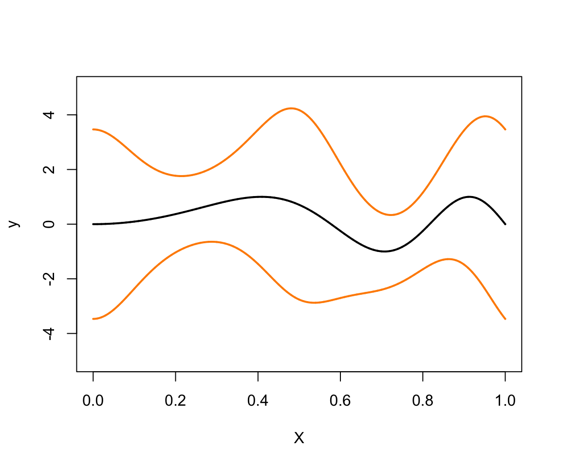
Expand here to see past versions of plot-mean-and-variance-1.png:
| Version | Author | Date |
|---|---|---|
| 613f9b2 | Peter Carbonetto | 2018-11-09 |
First simulation scenario: unevenly spaced data
In the first scenario, we simulate data sets with 500 unevenly spaced data points, and assess accuracy, separately for the mean and variance estimates) by computing the mean of the squared errors (MSE) evaluated at 201 equally spaced points.
mse.mu.uneven.mfvb  <- 0
mse.mu.uneven.smash <- 0
mse.sd.uneven.mfvb  <- 0
mse.sd.uneven.smash <- 0
Run the SMASH and MFVB methods for each simulated data set.
cat(sprintf("Running %d simulations: ",nsim1))
for (j in 1:nsim1) {
  cat(sprintf("%d ",j))

  # SIMULATE DATA
  set.seed(3*j)
  n     <- 500
  xOrig <- runif(n)
  set.seed(3*j)
  yOrig <- fTrue(xOrig) + sqrt(exp(loggTrue(xOrig)))*rnorm(n)

  aOrig  <- min(xOrig)
  bOrig  <- max(xOrig)
  mean.x <- mean(xOrig)
  sd.x   <- sd(xOrig)
  mean.y <- mean(yOrig)
  sd.y   <- sd(yOrig)

  a <- (aOrig - mean.x)/sd.x
  b <- (bOrig - mean.x)/sd.x
  x <- (xOrig - mean.x)/sd.x
  y <- (yOrig - mean.y)/sd.y

  numIntKnotsU <- 17
  intKnotsU <- quantile(x,seq(0,1,length=numIntKnotsU+2)[-c(1,numIntKnotsU+2)])
  Zu        <- ZOSull(x,intKnots=intKnotsU,range.x=c(a,b))
  numKnotsU <- ncol(Zu)

  numIntKnotsV <- numIntKnotsU
  intKnotsV <-
    quantile(x,seq(0,1,length = numIntKnotsV + 2)[-c(1,numIntKnotsV+2)])
  Zv        <- ZOSull(x,intKnots=intKnotsV,range.x=c(a,b))
  numKnotsV <- ncol(Zv)

  # RUN MEAN FIELD VARIATIONAL BAYES
  X     <- cbind(rep(1,n),x)
  Cumat <- cbind(X,Zu)
  Cvmat <- cbind(X,Zv)
  ncX   <- ncol(X)
  ncZu  <- ncol(Zu)
  ncZv  <- ncol(Zv)
  ncCu  <- ncol(Cumat)
  ncCv  <- ncol(Cvmat)

  MFVBfit <- meanVarMFVB(y,X,ncZu,ncZv,Au.hyp,Av.hyp,
                         sigsq.gamma,sigsq.beta)

  ng     <- 201
  xgOrig <- seq(aOrig,bOrig,length=ng)
  xg     <- (xgOrig - mean.x)/sd.x
  Xg     <- cbind(rep(1,ng),xg)
  Zug    <- ZOSull(xg,intKnots=intKnotsU,range.x=c(a,b))
  Cug    <- cbind(Xg,Zug)
  Zvg    <- ZOSull(xg,intKnots=intKnotsV,range.x=c(a,b))
  Cvg    <- cbind(Xg,Zvg)

  mu.q.nu       <- MFVBfit$mu.q.nu
  mu.q.omega    <- MFVBfit$mu.q.omega
  Sigma.q.nu    <- MFVBfit$Sigma.q.nu
  Sigma.q.omega <- MFVBfit$Sigma.q.omega

  fhatMFVBg        <- Cug%*%mu.q.nu
  fhatMFVBgOrig    <- fhatMFVBg*sd.y + mean.y
  logghatMFVBg     <- Cvg%*%mu.q.omega
  logghatMFVBgOrig <- logghatMFVBg + 2*log(sd.y)

  sdloggMFVBgOrig      <- sqrt(diag(Cvg%*%Sigma.q.omega%*%t(Cvg)))
  credLowloggMFVBgOrig <- logghatMFVBgOrig - qnorm(0.975)*sdloggMFVBgOrig
  credUpploggMFVBgOrig <- logghatMFVBgOrig + qnorm(0.975)*sdloggMFVBgOrig

  sqrtghatMFVBg     <- exp(0.5*Cvg %*% mu.q.omega
                           + 0.125*diag(Cvg%*%Sigma.q.omega%*%t(Cvg)))
  sqrtghatMFVBgOrig <- sqrtghatMFVBg*sd.y

  # RUN SMASH
  x.mod <- unique(sort(xOrig))
  y.mod <- 0
  for(i in 1:length(x.mod))
    y.mod[i] <- median(yOrig[xOrig == x.mod[i]])

  y.exp   <- c(y.mod,y.mod[length(y.mod):(2*length(y.mod)-2^9+1)])
  y.final <- c(y.exp,y.exp[length(y.exp):1])

  mu.est  <- smash.gaus(y.final,filter.number=1,family="DaubExPhase")
  var.est <- smash.gaus(y.final,v.est=TRUE)
  mu.est  <- mu.est[1:500]
  var.est <- var.est[1:500]

  mu.est.inter  <- approx(x.mod,mu.est,xgOrig,'linear')$y
  var.est.inter <- approx(x.mod,var.est,xgOrig,'linear')$y

  mse.mu.uneven.mfvb[j]<-mean((fhatMFVBgOrig - fTrue(xgOrig))^2)
  mse.sd.uneven.mfvb[j]<-mean((sqrtghatMFVBgOrig-exp((loggTrue(xgOrig))/2))^2)

  mu.est  <- smash.gaus(y.final,filter.number=8,family="DaubLeAsymm")
  var.est <- smash.gaus(y.final,v.est=TRUE,v.basis=TRUE,filter.number=8,
                        family="DaubLeAsymm")

  mu.est  <- mu.est[1:500]
  var.est <- var.est[1:500]

  mu.est.inter       <- approx(x.mod,mu.est,xgOrig,'linear')$y
  var.est.inter      <- approx(x.mod,var.est,xgOrig,'linear')$y

  mse.mu.uneven.smash[j] <- mean((mu.est.inter-fTrue(xgOrig))^2)
  mse.sd.uneven.smash[j] <-
    mean((sqrt(var.est.inter)-exp((loggTrue(xgOrig))/2))^2)
}
# Running 100 simulations: 1 2 3 4 5 6 7 8 9 10 11 12 13 14 15 16 17 18 19 20 21 22 23 24 25 26 27 28 29 30 31 32 33 34 35 36 37 38 39 40 41 42 43 44 45 46 47 48 49 50 51 52 53 54 55 56 57 58 59 60 61 62 63 64 65 66 67 68 69 70 71 72 73 74 75 76 77 78 79 80 81 82 83 84 85 86 87 88 89 90 91 92 93 94 95 96 97 98 99 100
Second simulation scenario: evenly spaced points
In this scenario, we simulate data sets with 1,024 evenly spaced data points. We assess accuracy separately for the mean and standard deviation as the mean of the MSEs evaluated at each of the locations.
mse.mu.even.mfvb  <- 0
mse.mu.even.smash <- 0
mse.sd.even.mfvb  <- 0
mse.sd.even.smash <- 0
Run the SMASH and MFVB methods for each simulated data set.
cat(sprintf("Running %d simulations: ",nsim2))
for (j in 1:nsim2) {
  cat(sprintf("%d ",j))

  # SIMULATE DATA
  n      <- 2^10
  xOrig  <- (1:n)/n
  set.seed(30*j)
  yOrig  <- fTrue(xOrig) + sqrt(exp(loggTrue(xOrig)))*rnorm(n)
  aOrig  <- min(xOrig)
  bOrig  <- max(xOrig)
  mean.x <- mean(xOrig)
  sd.x   <- sd(xOrig)
  mean.y <- mean(yOrig)
  sd.y   <- sd(yOrig)

  a <- (aOrig - mean.x)/sd.x
  b <- (bOrig - mean.x)/sd.x
  x <- (xOrig - mean.x)/sd.x
  y <- (yOrig - mean.y)/sd.y

  numIntKnotsU <- 17
  intKnotsU <- quantile(x,seq(0,1,length=numIntKnotsU+2)[-c(1,numIntKnotsU+2)])
  Zu        <- ZOSull(x,intKnots=intKnotsU,range.x=c(a,b))
  numKnotsU <- ncol(Zu)

  numIntKnotsV <- numIntKnotsU
  intKnotsV <- quantile(x,seq(0,1,length=numIntKnotsV+2)[-c(1,numIntKnotsV+2)])
  Zv        <- ZOSull(x,intKnots=intKnotsV,range.x=c(a,b))
  numKnotsV <- ncol(Zv)

  # RUN MEAN FIELD VARIATIONAL BAYES
  X     <- cbind(rep(1,n),x)
  Cumat <- cbind(X,Zu)
  Cvmat <- cbind(X,Zv)
  ncX   <- ncol(X)
  ncZu  <- ncol(Zu)
  ncZv  <- ncol(Zv)
  ncCu  <- ncol(Cumat)
  ncCv  <- ncol(Cvmat)

  MFVBfit <- meanVarMFVB(y,X,ncZu,ncZv,Au.hyp,Av.hyp,
                       sigsq.gamma,sigsq.beta)

  ng     <- 2^10
  xgOrig <- seq(aOrig,bOrig,length=ng)
  xg  <- (xgOrig - mean.x)/sd.x
  Xg  <- cbind(rep(1,ng),xg)
  Zug <- ZOSull(xg,intKnots=intKnotsU,range.x=c(a,b))
  Cug <- cbind(Xg,Zug)
  Zvg <- ZOSull(xg,intKnots=intKnotsV,range.x=c(a,b))
  Cvg <- cbind(Xg,Zvg)

  mu.q.nu       <- MFVBfit$mu.q.nu
  mu.q.omega    <- MFVBfit$mu.q.omega
  Sigma.q.nu    <- MFVBfit$Sigma.q.nu
  Sigma.q.omega <- MFVBfit$Sigma.q.omega

  # Get the mean function estimate.
  fhatMFVBg     <- Cug %*% mu.q.nu
  fhatMFVBgOrig <- fhatMFVBg*sd.y + mean.y

  logghatMFVBg     <- Cvg%*%mu.q.omega
  logghatMFVBgOrig <- logghatMFVBg + 2*log(sd.y)

  sdloggMFVBgOrig      <- sqrt(diag(Cvg%*%Sigma.q.omega%*%t(Cvg)))
  credLowloggMFVBgOrig <- logghatMFVBgOrig - qnorm(0.975)*sdloggMFVBgOrig
  credUpploggMFVBgOrig <- logghatMFVBgOrig + qnorm(0.975)*sdloggMFVBgOrig

  sqrtghatMFVBg     <- exp(0.5*Cvg%*%mu.q.omega
                           + 0.125*diag(Cvg%*%Sigma.q.omega%*%t(Cvg)))
  sqrtghatMFVBgOrig <- sqrtghatMFVBg*sd.y

  # RUN SMASH
  mu.est  <- smash.gaus(yOrig,filter.number=1,family="DaubExPhase")
  var.est <- smash.gaus(yOrig,v.est=TRUE)

  mse.mu.even.mfvb[j] <- mean((fhatMFVBgOrig-fTrue(xgOrig))^2)
  mse.sd.even.mfvb[j] <- mean((sqrtghatMFVBgOrig-exp((loggTrue(xgOrig))/2))^2)

  mu.est  <- smash.gaus(yOrig,filter.number=8,family="DaubLeAsymm")
  var.est <- smash.gaus(yOrig,v.est=TRUE,v.basis=TRUE,filter.number=8,
                        family = "DaubLeAsymm")

  mse.mu.even.smash[j]  <- mean((mu.est - fTrue(xgOrig))^2)
  mse.sd.even.smash[j]  <- mean((sqrt(var.est)-exp((loggTrue(xgOrig))/2))^2)
}
# Running 100 simulations: 1 2 3 4 5 6 7 8 9 10 11 12 13 14 15 16 17 18 19 20 21 22 23 24 25 26 27 28 29 30 31 32 33 34 35 36 37 38 39 40 41 42 43 44 45 46 47 48 49 50 51 52 53 54 55 56 57 58 59 60 61 62 63 64 65 66 67 68 69 70 71 72 73 74 75 76 77 78 79 80 81 82 83 84 85 86 87 88 89 90 91 92 93 94 95 96 97 98 99 100
Summarize results of simulations
The following two tables show the mean squared error (MSE) averaged over the 100 simulations in each of the scenarios. Compare these results with Table 1 in the paper.
mse.table1 <- rbind(c(mean(mse.mu.uneven.mfvb),mean(mse.sd.uneven.mfvb)),
                    c(mean(mse.mu.uneven.smash),mean(mse.sd.uneven.smash)))
mse.table2 <- rbind(c(mean(mse.mu.even.mfvb),mean(mse.sd.even.mfvb)),
                    c(mean(mse.mu.even.smash),mean(mse.sd.even.smash)))
rownames(mse.table1) <- c("MFVB","SMASH")
colnames(mse.table1) <- c("mean","sd")
rownames(mse.table2) <- c("MFVB","SMASH")
colnames(mse.table2) <- c("mean","sd")
cat(sprintf("MSE averaged across %d simulations in Scenario 1:\n",nsim1))
print(mse.table1)
cat("\n")
cat(sprintf("MSE averaged across %d simulations in Scenario 2:\n",nsim2))
print(mse.table2)
# MSE averaged across 100 simulations in Scenario 1:
#             mean         sd
# MFVB  0.03302778 0.01991272
# SMASH 0.03343833 0.01869602
#
# MSE averaged across 100 simulations in Scenario 2:
#             mean          sd
# MFVB  0.01721438 0.008471983
# SMASH 0.01582035 0.006513889
In Scenario 1, the data are not equally spaced, and the number of data points is not a power of 2; in this setting, SMASH is more accurate in estimating both the mean and s.d.
In Scenario 2, the data are equally spaced, and the number of data points is a power of 2; SMASH again outperforms MFVB in both mean and s.d. estimation.
Session information
sessionInfo()
# R version 3.4.3 (2017-11-30)
# Platform: x86_64-apple-darwin15.6.0 (64-bit)
# Running under: macOS High Sierra 10.13.6
#
# Matrix products: default
# BLAS: /Library/Frameworks/R.framework/Versions/3.4/Resources/lib/libRblas.0.dylib
# LAPACK: /Library/Frameworks/R.framework/Versions/3.4/Resources/lib/libRlapack.dylib
#
# locale:
# [1] en_US.UTF-8/en_US.UTF-8/en_US.UTF-8/C/en_US.UTF-8/en_US.UTF-8
#
# attached base packages:
# [1] splines   stats     graphics  grDevices utils     datasets  methods
# [8] base
#
# other attached packages:
# [1] smashr_1.2-0
#
# loaded via a namespace (and not attached):
#  [1] Rcpp_0.12.19      compiler_3.4.3    git2r_0.23.0
#  [4] workflowr_1.1.1   R.methodsS3_1.7.1 R.utils_2.6.0
#  [7] bitops_1.0-6      iterators_1.0.9   tools_3.4.3
# [10] digest_0.6.17     evaluate_0.11     lattice_0.20-35
# [13] Matrix_1.2-12     foreach_1.4.4     yaml_2.2.0
# [16] parallel_3.4.3    stringr_1.3.1     knitr_1.20
# [19] caTools_1.17.1    REBayes_1.3       rprojroot_1.3-2
# [22] grid_3.4.3        data.table_1.11.4 rmarkdown_1.10
# [25] ashr_2.2-23       magrittr_1.5      whisker_0.3-2
# [28] backports_1.1.2   codetools_0.2-15  htmltools_0.3.6
# [31] MASS_7.3-48       assertthat_0.2.0  wavethresh_4.6.8
# [34] stringi_1.2.4     Rmosek_8.0.69     doParallel_1.0.11
# [37] pscl_1.5.2        truncnorm_1.0-8   SQUAREM_2017.10-1
# [40] R.oo_1.21.0
This reproducible R Markdown analysis was created with workflowr 1.1.1