Please add a more descriptive title
Sarah Urbut
Last updated: 2018-05-09
workflowr checks: (Click a bullet for more information)-
✖ R Markdown file: uncommitted changes
The R Markdown file has unstaged changes. To know which version of the R Markdown file created these results, you’ll want to first commit it to the Git repo. If you’re still working on the analysis, you can ignore this warning. When you’re finished, you can runwflow_publishto commit the R Markdown file and build the HTML. -
✔ Environment: empty
Great job! The global environment was empty. Objects defined in the global environment can affect the analysis in your R Markdown file in unknown ways. For reproduciblity it’s best to always run the code in an empty environment.
-
✔ Seed:
set.seed(1)The command
set.seed(1)was run prior to running the code in the R Markdown file. Setting a seed ensures that any results that rely on randomness, e.g. subsampling or permutations, are reproducible. -
✔ Session information: recorded
Great job! Recording the operating system, R version, and package versions is critical for reproducibility.
-
Great! You are using Git for version control. Tracking code development and connecting the code version to the results is critical for reproducibility. The version displayed above was the version of the Git repository at the time these results were generated.✔ Repository version: ea42e8a
Note that you need to be careful to ensure that all relevant files for the analysis have been committed to Git prior to generating the results (you can usewflow_publishorwflow_git_commit). workflowr only checks the R Markdown file, but you know if there are other scripts or data files that it depends on. Below is the status of the Git repository when the results were generated:
Note that any generated files, e.g. HTML, png, CSS, etc., are not included in this status report because it is ok for generated content to have uncommitted changes.Ignored files: Ignored: .sos/ Ignored: data/.sos/ Ignored: workflows/.ipynb_checkpoints/ Ignored: workflows/.sos/ Untracked files: Untracked: gtex6_workflow_output/ Unstaged changes: Modified: analysis/Fig.Uk3.Rmd
Expand here to see past versions:
“Uk3” is the covariance matrix corresponding to the output of the ExtremeDeconvolution algorithm that was initialized with the rank3 SVD approximation of \(X^TX\). It is the pattern of sharing with the most loading. We demonstrate which patterns have the most loading the \(\pi\) barplot.
We plot the correlation matrix and the first 3 eigenvectors of “Uk3”. This provides a visualization of the primary patterns of genetic sharing identified by our method, mash. It is also Fig. 3 in the paper.
Set up environment
First, we load some packages into the R environment.
library(lattice)
library(ggplot2)
library(colorRamps)
library(fields)
Load data
Next, we load data generated
Explain here what this next code chunk does. It looks like you are loading a bunch of data sets from files. What are these data sets? And what is the bar chart you are creating?
# Files generated by Gao's analysis pipeline:
# covmat <- readRDS(paste0("../gtex6_workflow_output/MatrixEQTLSumStats.",
#                          "Portable.Z.coved.K3.P3.lite.single.expanded.",
#                          "rds"))$covmat
# pis    <- readRDS(paste0("../gtex6_workflow_output/MatrixEQTLSumStats.",
#                          "Portable.Z.coved.K3.P3.lite.single.expanded.",
#                          "pihat.rds"))$pihat
covmat <- readRDS("../output/covmatwithvhat.rds")

z.stat <- read.table("../output/maxz.txt")
pis    <- readRDS("../output/piswithvhat.rds")$pihat
pi.mat <- matrix(pis[-length(pis)],ncol = 54,nrow = 22,byrow = TRUE)
names  <- colnames(z.stat)
colnames(pi.mat) <-
  c("ID","X'X","SVD","F1","F2","F3","F4","F5","SFA_Rank5",names,"ALL")

# Please label the horizontal and vertical axes.
barplot(colSums(pi.mat),las = 2,cex.names = 0.5)
Here, we load the indices (of the tissues?) and tissue names:
k <- 3

x           <- cov2cor(covmat[[k]])
x[x < 0]    <- 0
colnames(x) <- names
rownames(x) <- names

h <- read.table("../output/uk3rowindices.txt")[,1]
Now we produce the heatmap. What is the heat map showing? What interesting result(s) are highlighted by this heat map? Note that this is flipped in the paper:
smat <- (x[(h),(h)])
smat[lower.tri(smat)] <- NA

clrs <- colorRampPalette(rev(c("#D73027","#FC8D59","#FEE090","#FFFFBF",
                               "#E0F3F8","#91BFDB","#4575B4")))(64)
lat <- x[rev(h),rev(h)]

lat[lower.tri(lat)] <- NA
n <- nrow(lat)
print(levelplot(lat[n:1,],col.regions = clrs,xlab = "",ylab = "",
                colorkey = TRUE,at = seq(0,1,length.out = 64),
                scales = list(cex = 0.6,x = list(rot = 45))))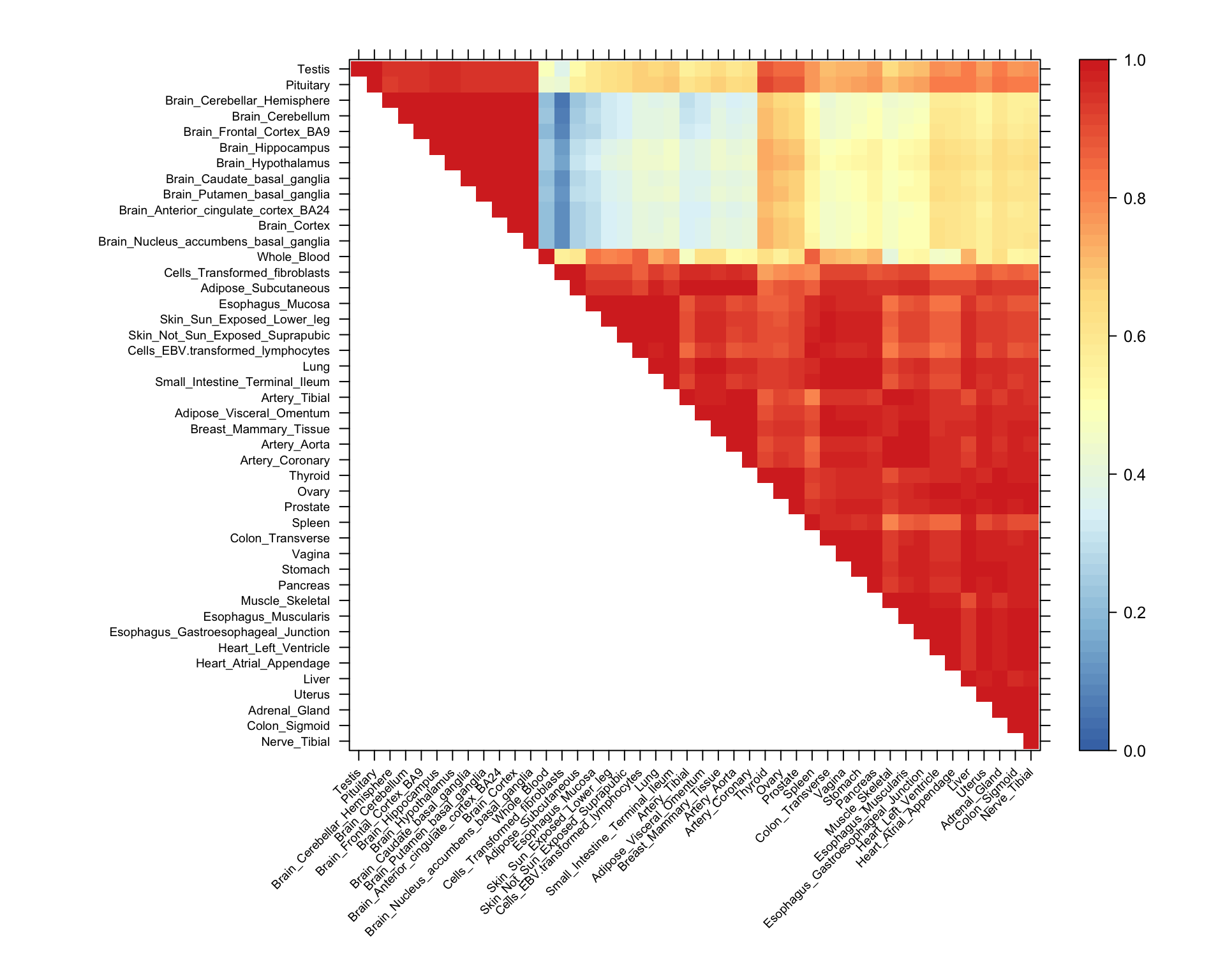
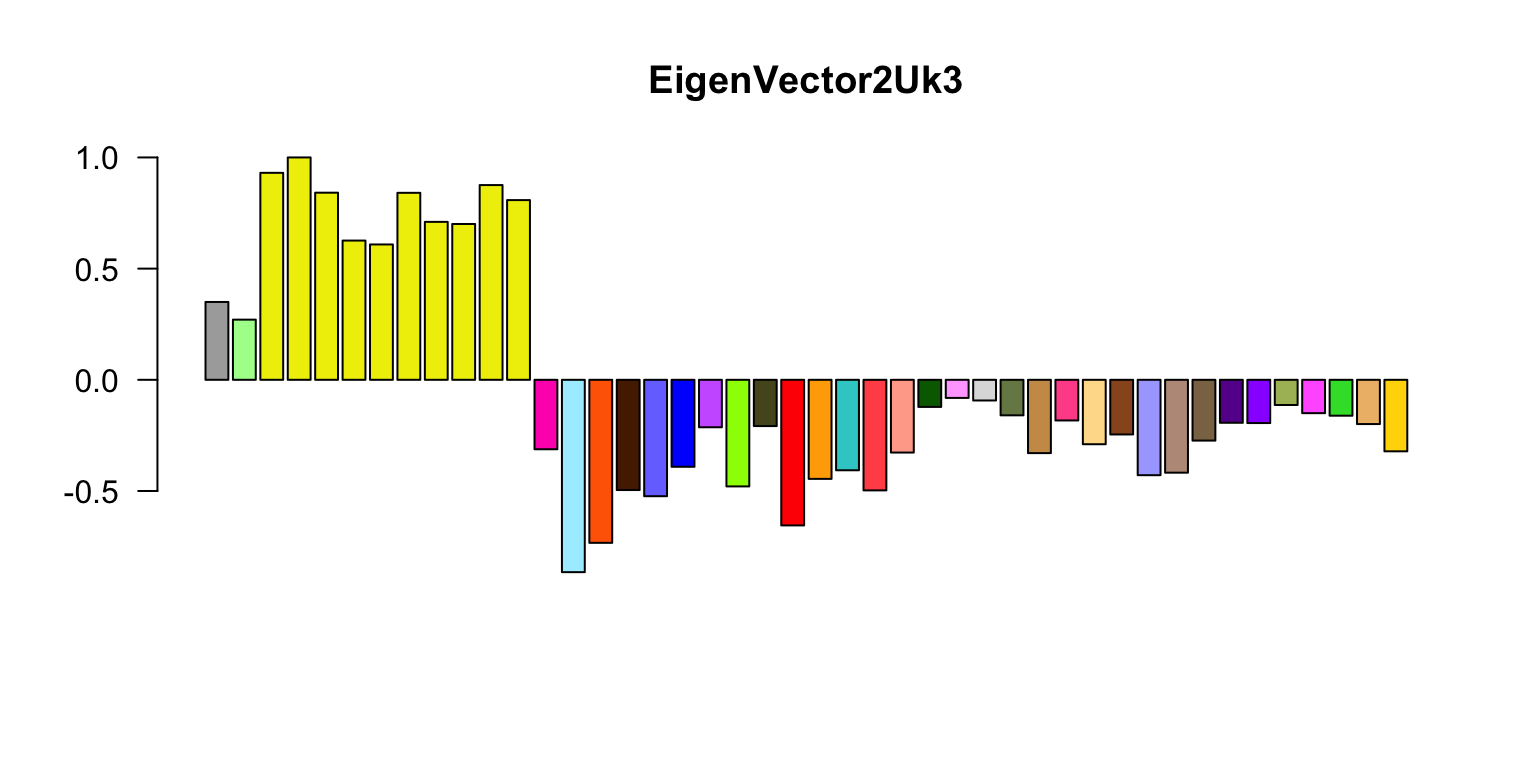
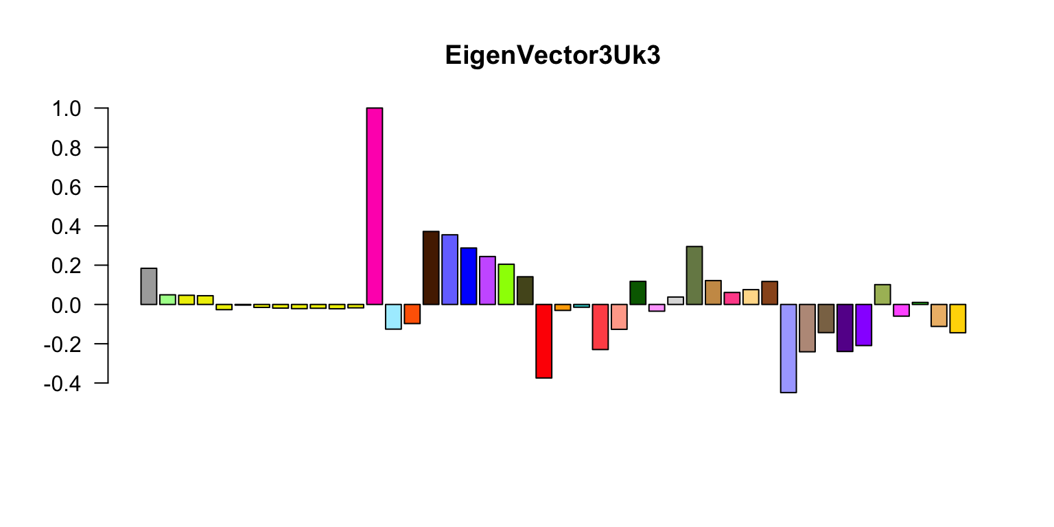
Now let’s do the eigenplots. What are these plots showing, and what sort of interesting results (briefly) are being highlighted by these plots? Can you briefly explain the color scheme you are using?
missing.tissues <- c(7,8,19,20,24,25,31,34,37)
color.gtex <- read.table("../Data/GTExColors.txt",sep = "\t",
                         comment.char = '')[-missing.tissues,]
k <- 3
vold  <- svd(covmat[[k]])$v
u     <- svd(covmat[[k]])$u
d     <- svd(covmat[[k]])$d
v     <- vold[h,] # Shuffle so correct order
names <- names[h]
color.gtex <- color.gtex[h,]
for (j in 1:3)

  # Please add labels to the horizontal and vertical axes in these plots.
  barplot(v[,j]/v[,j][which.max(abs(v[,j]))],names = "",cex.names = 0.5,
          las = 2,main = paste0("EigenVector",j,"Uk",k),
          col = as.character(color.gtex[,2]))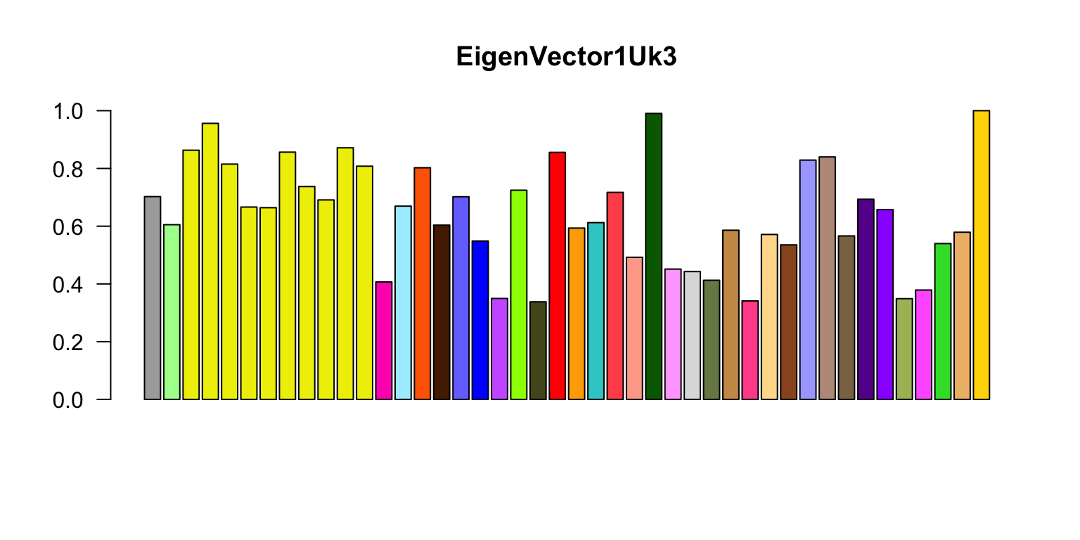
Session information
sessionInfo()
R version 3.4.3 (2017-11-30)
Platform: x86_64-apple-darwin15.6.0 (64-bit)
Running under: macOS High Sierra 10.13.4

Matrix products: default
BLAS: /Library/Frameworks/R.framework/Versions/3.4/Resources/lib/libRblas.0.dylib
LAPACK: /Library/Frameworks/R.framework/Versions/3.4/Resources/lib/libRlapack.dylib

locale:
[1] en_US.UTF-8/en_US.UTF-8/en_US.UTF-8/C/en_US.UTF-8/en_US.UTF-8

attached base packages:
[1] grid      stats     graphics  grDevices utils     datasets  methods
[8] base

other attached packages:
[1] fields_9.0      maps_3.2.0      spam_2.1-2      dotCall64_0.9-5
[5] colorRamps_2.3  ggplot2_2.2.1   lattice_0.20-35

loaded via a namespace (and not attached):
 [1] Rcpp_0.12.16         knitr_1.20           whisker_0.3-2
 [4] magrittr_1.5         workflowr_1.0.1.9000 munsell_0.4.3
 [7] colorspace_1.3-2     rlang_0.2.0.9000     stringr_1.3.0
[10] plyr_1.8.4           tools_3.4.3          gtable_0.2.0
[13] R.oo_1.21.0          git2r_0.21.0         htmltools_0.3.6
[16] lazyeval_0.2.1       yaml_2.1.18          rprojroot_1.3-2
[19] digest_0.6.15        tibble_1.4.2         R.utils_2.6.0
[22] evaluate_0.10.1      rmarkdown_1.9        stringi_1.1.7
[25] pillar_1.2.1         compiler_3.4.3       scales_0.5.0
[28] backports_1.1.2      R.methodsS3_1.7.1
This reproducible R Markdown analysis was created with workflowr 1.0.1.9000