Comparison of genes with tissue-specific eQTLs against other genes
Sarah Urbut, Gao Wang, Peter Carbonetto and Matthew Stephens
Last updated: 2018-06-05
workflowr checks: (Click a bullet for more information)-
✔ R Markdown file: up-to-date
Great! Since the R Markdown file has been committed to the Git repository, you know the exact version of the code that produced these results.
-
✔ Environment: empty
Great job! The global environment was empty. Objects defined in the global environment can affect the analysis in your R Markdown file in unknown ways. For reproduciblity it’s best to always run the code in an empty environment.
-
✔ Seed:
set.seed(1)The command
set.seed(1)was run prior to running the code in the R Markdown file. Setting a seed ensures that any results that rely on randomness, e.g. subsampling or permutations, are reproducible. -
✔ Session information: recorded
Great job! Recording the operating system, R version, and package versions is critical for reproducibility.
-
Great! You are using Git for version control. Tracking code development and connecting the code version to the results is critical for reproducibility. The version displayed above was the version of the Git repository at the time these results were generated.✔ Repository version: 4a93c87
Note that you need to be careful to ensure that all relevant files for the analysis have been committed to Git prior to generating the results (you can usewflow_publishorwflow_git_commit). workflowr only checks the R Markdown file, but you know if there are other scripts or data files that it depends on. Below is the status of the Git repository when the results were generated:
Note that any generated files, e.g. HTML, png, CSS, etc., are not included in this status report because it is ok for generated content to have uncommitted changes.Ignored files: Ignored: .sos/ Ignored: data/.sos/ Ignored: output/MatrixEQTLSumStats.Portable.Z.coved.K3.P3.lite.single.expanded.V1.loglik.rds Ignored: workflows/.ipynb_checkpoints/ Ignored: workflows/.sos/ Untracked files: Untracked: analysis/files.txt Untracked: fastqtl_to_mash_output/ Untracked: gtex6_workflow_output/ Unstaged changes: Modified: analysis/gtex.Rmd
Expand here to see past versions:
| File | Version | Author | Date | Message |
|---|---|---|---|---|
| Rmd | 4a93c87 | Peter Carbonetto | 2018-06-05 | wflow_publish(“ExpressionAnalysis.Rmd”) |
| html | 19b5442 | Peter Carbonetto | 2018-06-05 | Build site. |
| Rmd | 0a5d3bc | Peter Carbonetto | 2018-06-05 | Renamed Fig.ExpressionAnalysis.Rmd as ExpressionAnalysis.Rmd. |
| html | 0a5d3bc | Peter Carbonetto | 2018-06-05 | Renamed Fig.ExpressionAnalysis.Rmd as ExpressionAnalysis.Rmd. |
| html | afc401f | Peter Carbonetto | 2017-09-20 | Moved doc to docs. |
| Rmd | e1e48df | Peter Carbonetto | 2017-09-20 | Reorganized many of the files. |
In this analysis, we assess whether tissue-specific eQTLs we identified can be explained by tissue-specific expression. Specifically, we take genes with tissue-specific eQTLs, and examine the distribution of expression in the eQTL-affected tissue relative to expression in other tissues.
Load data and mash results
In the next code chunk, we load some GTEx summary statistics (average gene expression values and z-scores), as well as some of the results generated from the mash analysis of the GTEx data.
Expression is here defined as median across individuals of the log Reads per Kilobase Mapped (RPKM).
data <- read.csv("../data/AvgExpr.csv.gz",header = TRUE)
out  <- readRDS("../data/MatrixEQTLSumStats.Portable.Z.rds")
maxz <- out$test.z
qtl.names <-
  sapply(1:length(rownames(maxz)),
         function(x) unlist(strsplit(rownames(maxz)[x], "[_]"))[[1]])
rownames(data) <- data[,1]
expr.data      <- data[,-1]
out    <- readRDS(paste("../output/MatrixEQTLSumStats.Portable.Z.coved.K3.P3",
                        "lite.single.expanded.V1.posterior.rds",sep = "."))
pmash <- out$posterior.means
lfsr  <- out$lfsr
colnames(lfsr) <- colnames(pmash) <- colnames(maxz)
rownames(lfsr) <- rownames(pmash) <- rownames(maxz)
expr.sort <- expr.data[rownames(expr.data)%in%qtl.names,]
a         <- match(qtl.names,rownames(expr.sort))
expr.sort <- expr.sort[a,]
missing.tissues    <- c(7,8,19,20,24,25,31,34,37)
exp.sort           <- expr.sort[,-missing.tissues]
colnames(exp.sort) <- colnames(maxz)
Define plotting functions
Here we define a couple functions used to compare the densities and CDFs of gene expression levels.
plot_tissuespecifictwo = function(tissuename,lfsr,ymax,curvedata,title,
                                  thresh=0.05,subset=1:44,exclude=0.01) {
  index_tissue=which(colnames(lfsr) %in% tissuename);
  ybar=title

  # Create a matrix showing whether or not lfsr satisfies threshold.
  sigmat = lfsr <= thresh;
  sigs=which(rowSums(sigmat[,index_tissue,drop=FALSE])==length(tissuename) &
             rowSums(sigmat[,-index_tissue,drop=FALSE])==0)
  norm.spec=density(curvedata[sigs,index_tissue])
  norm.other=density(curvedata[-sigs,index_tissue])
  xmin=min(norm.spec$x,norm.other$x)-1
  ymin=min(norm.spec$y,norm.other$y)
  xmax=max(norm.spec$x,norm.other$x)+1

  plot(norm.other,xlim = c(xmin,xmax),ylim=c(0,ymax),
       col="black",main=tissuename,xlab="log(RPKM)")

  lines(norm.spec,col="red")
  legend("right",legend = c("All Genes","Tissue Specific"),
         col=c("black","red"),pch=c(1,1))
  }

plot_tissuespecificthree = function(tissuename,lfsr,ymax,curvedata,title,
                                    thresh=0.05,subset=1:44,exclude=0.01) {
  index_tissue=which(colnames(lfsr) %in% tissuename);
  ybar=title

  # Create a matrix showing whether or not lfsr satisfies threshold.
  sigmat = lfsr <= thresh
  sigs=which(rowSums(sigmat[,index_tissue,drop=FALSE])==length(tissuename) &
             rowSums(sigmat[,-index_tissue,drop=FALSE])==0)
  norm.spec=ecdf(curvedata[sigs,index_tissue])
  norm.other=ecdf(curvedata[-sigs,index_tissue])
  plot(norm.other,ylim=c(0,ymax),
       col="black",main=tissuename,xlab="log(RPKM)")

    lines(norm.spec,col="red",cex=0.1)
    legend("right",legend = c("All Genes","Tissue Specific"),
           col=c("black","red"),pch=c(1,1))
  }
Distribution of expression levels in testis
The two plots below compare the densities and cumulative distribution functions of the expression levels for all genes (black), and for genes identified as having a “tissue-specific” eQTL (red) in testis.
plot_tissuespecifictwo(tissuename = "Testis",lfsr = lfsr,
                       curvedata = log(exp.sort),title = "Test",
                       thresh = 0.05 ,ymax=0.5)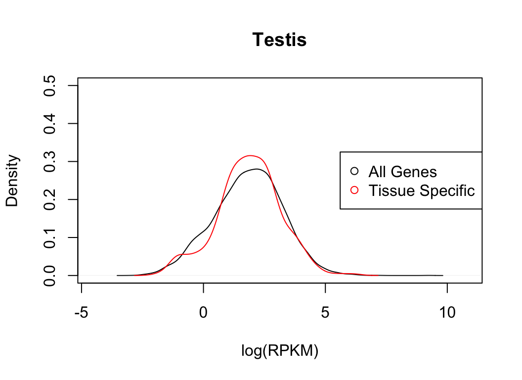
Expand here to see past versions of testis-1.png:
| Version | Author | Date |
|---|---|---|
| 0a5d3bc | Peter Carbonetto | 2018-06-05 |
plot_tissuespecificthree(tissuename = "Testis",lfsr = lfsr,
                         curvedata = log(exp.sort),title = "Test",
                         thresh = 0.05 ,ymax=1)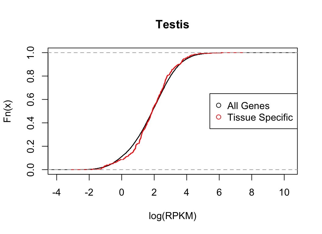
Expand here to see past versions of testis-2.png:
| Version | Author | Date |
|---|---|---|
| 0a5d3bc | Peter Carbonetto | 2018-06-05 |
The distribution functions are reasonably similar.
Distribution of expression levels in thyroid
Next we show the same two plots for thyroid.
plot_tissuespecifictwo(tissuename = "Thyroid",lfsr = lfsr,
                       curvedata = log(exp.sort),title = "Test",
                       thresh = 0.05,ymax = 0.5)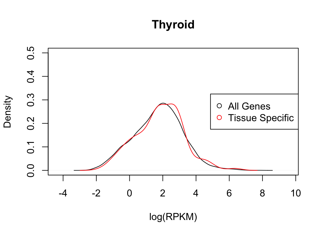
Expand here to see past versions of thyroid-1.png:
| Version | Author | Date |
|---|---|---|
| 0a5d3bc | Peter Carbonetto | 2018-06-05 |
plot_tissuespecificthree(tissuename = "Thyroid",lfsr = lfsr,
                         curvedata = log(exp.sort),title = "Test",
                         thresh = 0.05,ymax = 1)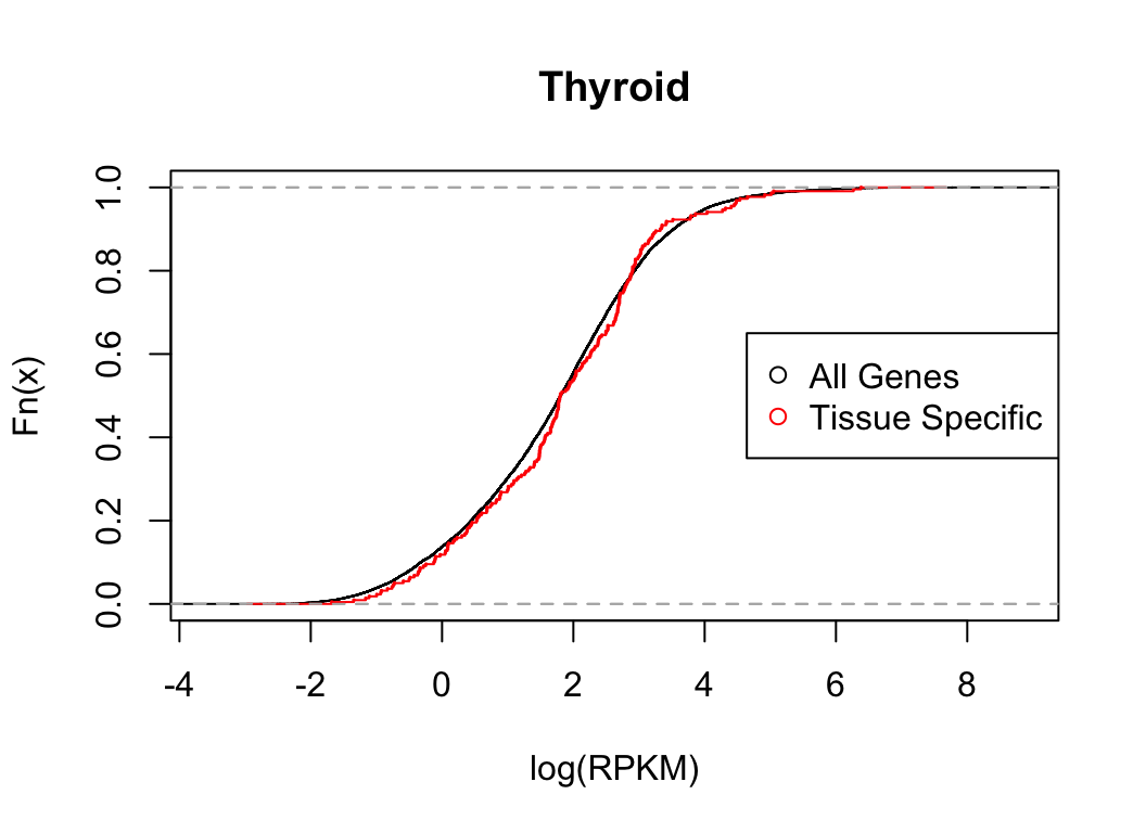
Expand here to see past versions of thyroid-2.png:
| Version | Author | Date |
|---|---|---|
| 0a5d3bc | Peter Carbonetto | 2018-06-05 |
Distribution of expression levels in whole blood
Next, we look at the distributions in whole blood cells.
plot_tissuespecifictwo(tissuename = "Whole_Blood",lfsr = lfsr,
                       curvedata = log(exp.sort),title = "Test",
                       thresh = 0.05,ymax=0.5)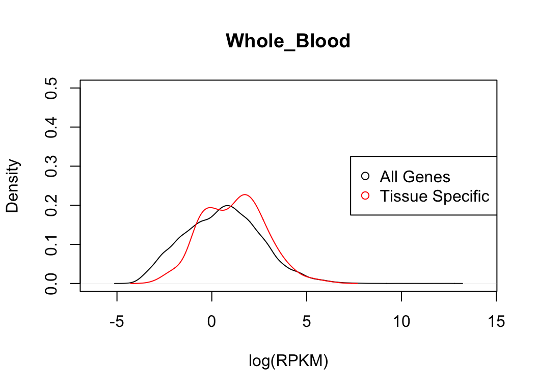
Expand here to see past versions of whole-blood-1.png:
| Version | Author | Date |
|---|---|---|
| 0a5d3bc | Peter Carbonetto | 2018-06-05 |
plot_tissuespecificthree(tissuename = "Whole_Blood",lfsr = lfsr,
                         curvedata = log(exp.sort),title = "Test",
                         thresh = 0.05 ,ymax=1)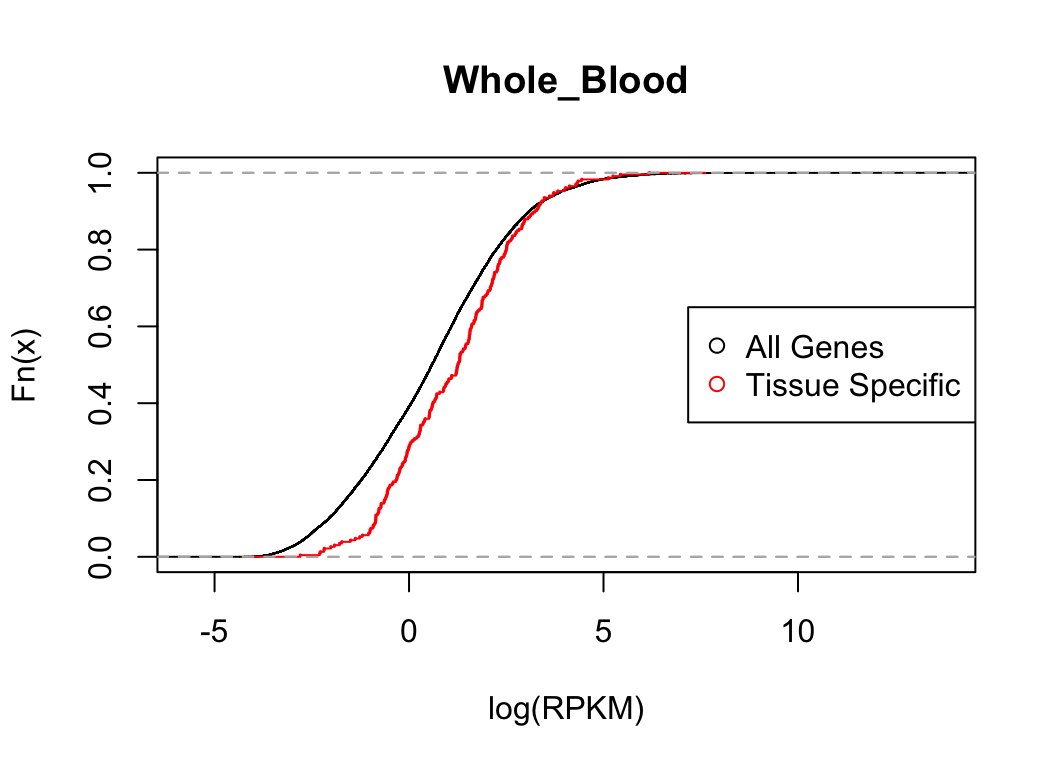
Expand here to see past versions of whole-blood-2.png:
| Version | Author | Date |
|---|---|---|
| 0a5d3bc | Peter Carbonetto | 2018-06-05 |
Distribution of expression levels in fibroblasts
Finally, we examine the gene expression distributions in fibroblasts.
plot_tissuespecifictwo(tissuename = "Cells_Transformed_fibroblasts",
                       lfsr = lfsr,curvedata = log(exp.sort),title = "Test",
                       thresh = 0.05,ymax=0.5)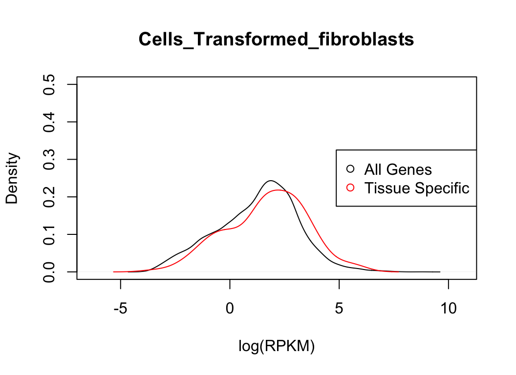
Expand here to see past versions of fibroblasts-1.png:
| Version | Author | Date |
|---|---|---|
| 0a5d3bc | Peter Carbonetto | 2018-06-05 |
plot_tissuespecificthree(tissuename = "Cells_Transformed_fibroblasts",
                        lfsr = lfsr,curvedata = log(exp.sort),title = "Test",
                        thresh = 0.05 ,ymax=1)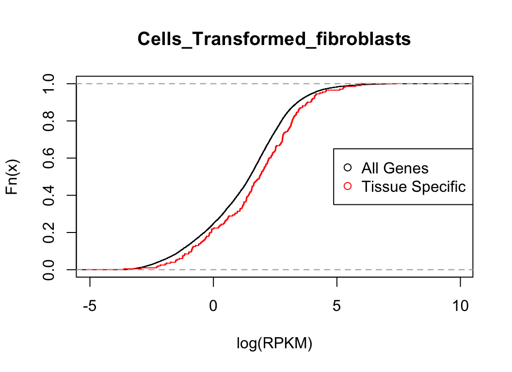
Expand here to see past versions of fibroblasts-2.png:
| Version | Author | Date |
|---|---|---|
| 0a5d3bc | Peter Carbonetto | 2018-06-05 |
In each case, the distribution functions are similar. This tells us that tissue-specific eQTLs are not simply reflecting tissue-specific expression.
Session information
sessionInfo()
# R version 3.4.3 (2017-11-30)
# Platform: x86_64-apple-darwin15.6.0 (64-bit)
# Running under: macOS High Sierra 10.13.4
#
# Matrix products: default
# BLAS: /Library/Frameworks/R.framework/Versions/3.4/Resources/lib/libRblas.0.dylib
# LAPACK: /Library/Frameworks/R.framework/Versions/3.4/Resources/lib/libRlapack.dylib
#
# locale:
# [1] en_US.UTF-8/en_US.UTF-8/en_US.UTF-8/C/en_US.UTF-8/en_US.UTF-8
#
# attached base packages:
# [1] stats     graphics  grDevices utils     datasets  methods   base
#
# loaded via a namespace (and not attached):
#  [1] workflowr_1.0.1.9000 Rcpp_0.12.16         digest_0.6.15
#  [4] rprojroot_1.3-2      R.methodsS3_1.7.1    backports_1.1.2
#  [7] git2r_0.21.0         magrittr_1.5         evaluate_0.10.1
# [10] stringi_1.1.7        whisker_0.3-2        R.oo_1.21.0
# [13] R.utils_2.6.0        rmarkdown_1.9        tools_3.4.3
# [16] stringr_1.3.0        yaml_2.1.18          compiler_3.4.3
# [19] htmltools_0.3.6      knitr_1.20
This reproducible R Markdown analysis was created with workflowr 1.0.1.9000