Pairwise sharing by magnitude of eQTLs among tissues
Sarah Urbut
Last updated: 2018-05-22
workflowr checks: (Click a bullet for more information)-
✔ R Markdown file: up-to-date
Great! Since the R Markdown file has been committed to the Git repository, you know the exact version of the code that produced these results.
-
✔ Environment: empty
Great job! The global environment was empty. Objects defined in the global environment can affect the analysis in your R Markdown file in unknown ways. For reproduciblity it’s best to always run the code in an empty environment.
-
✔ Seed:
set.seed(1)The command
set.seed(1)was run prior to running the code in the R Markdown file. Setting a seed ensures that any results that rely on randomness, e.g. subsampling or permutations, are reproducible. -
✔ Session information: recorded
Great job! Recording the operating system, R version, and package versions is critical for reproducibility.
-
Great! You are using Git for version control. Tracking code development and connecting the code version to the results is critical for reproducibility. The version displayed above was the version of the Git repository at the time these results were generated.✔ Repository version: 6ca4127
Note that you need to be careful to ensure that all relevant files for the analysis have been committed to Git prior to generating the results (you can usewflow_publishorwflow_git_commit). workflowr only checks the R Markdown file, but you know if there are other scripts or data files that it depends on. Below is the status of the Git repository when the results were generated:
Note that any generated files, e.g. HTML, png, CSS, etc., are not included in this status report because it is ok for generated content to have uncommitted changes.Ignored files: Ignored: .sos/ Ignored: data/.sos/ Ignored: workflows/.ipynb_checkpoints/ Ignored: workflows/.sos/ Untracked files: Untracked: gtex6_workflow_output/ Unstaged changes: Modified: analysis/Fig.GTExExamples.Rmd
Expand here to see past versions:
The plot generated here summarizes eQTL sharing by magnitude between all pairs of tissues. Compare against Figure 6 of the paper.
Set up environment
First, we load the lattice package used for generating the plot below.
library(lattice)Load data and MASH results
In the next code chunk, we load some GTEx summary statistics, as well as some of the results generated from the MASH analysis of the GTEx data.
out      <- readRDS("../data/MatrixEQTLSumStats.Portable.Z.rds")
maxb     <- out$test.b
maxz     <- out$test.z
out      <-readRDS(paste("../output/MatrixEQTLSumStats.Portable.Z.coved.K3.P3",
                         "lite.single.expanded.V1.posterior.rds",sep = "."))
pm.mash  <- out$posterior.means
lfsr.all <- out$lfsr
standard.error <- maxb/maxz
pm.mash.beta <- pm.mash*standard.error
Compute sharing-by-magnitude statistics
For every pair of tissues, we count the proportion of effects significant in either tissue that are within 2-fold magnitude of one another.
thresh <- 0.05
pm.mash.beta <- pm.mash.beta[rowSums(lfsr.all<0.05)>0,]
lfsr.mash <- lfsr.all[rowSums(lfsr.all<0.05)>0,]
shared.fold.size <- matrix(NA,nrow = ncol(lfsr.mash),ncol=ncol(lfsr.mash))
colnames(shared.fold.size) <- rownames(shared.fold.size) <- colnames(maxz)
for (i in 1:ncol(lfsr.mash))
for (j in 1:ncol(lfsr.mash)) {
sig.row=which(lfsr.mash[,i]<thresh)
sig.col=which(lfsr.mash[,j]<thresh)
a=(union(sig.row,sig.col))
quotient=(pm.mash.beta[a,i]/pm.mash.beta[a,j])##divide effect sizes
shared.fold.size[i,j]=mean(quotient>0.5"ient<2)
}Generate the heatmap using the “levelplot” function from the lattice package.
all.tissue.order <- read.table("../output/alltissueorder.txt")[,1]
clrs <- colorRampPalette(rev(c("#D73027","#FC8D59","#FEE090","#FFFFBF",
                               "#E0F3F8","#91BFDB","#4575B4")))(64)
lat <- shared.fold.size[rev(all.tissue.order),rev(all.tissue.order)]
lat[lower.tri(lat)] <- NA
n <- nrow(lat)
print(levelplot(lat[n:1,],col.regions = clrs,xlab = "",ylab = "",
      colorkey = TRUE))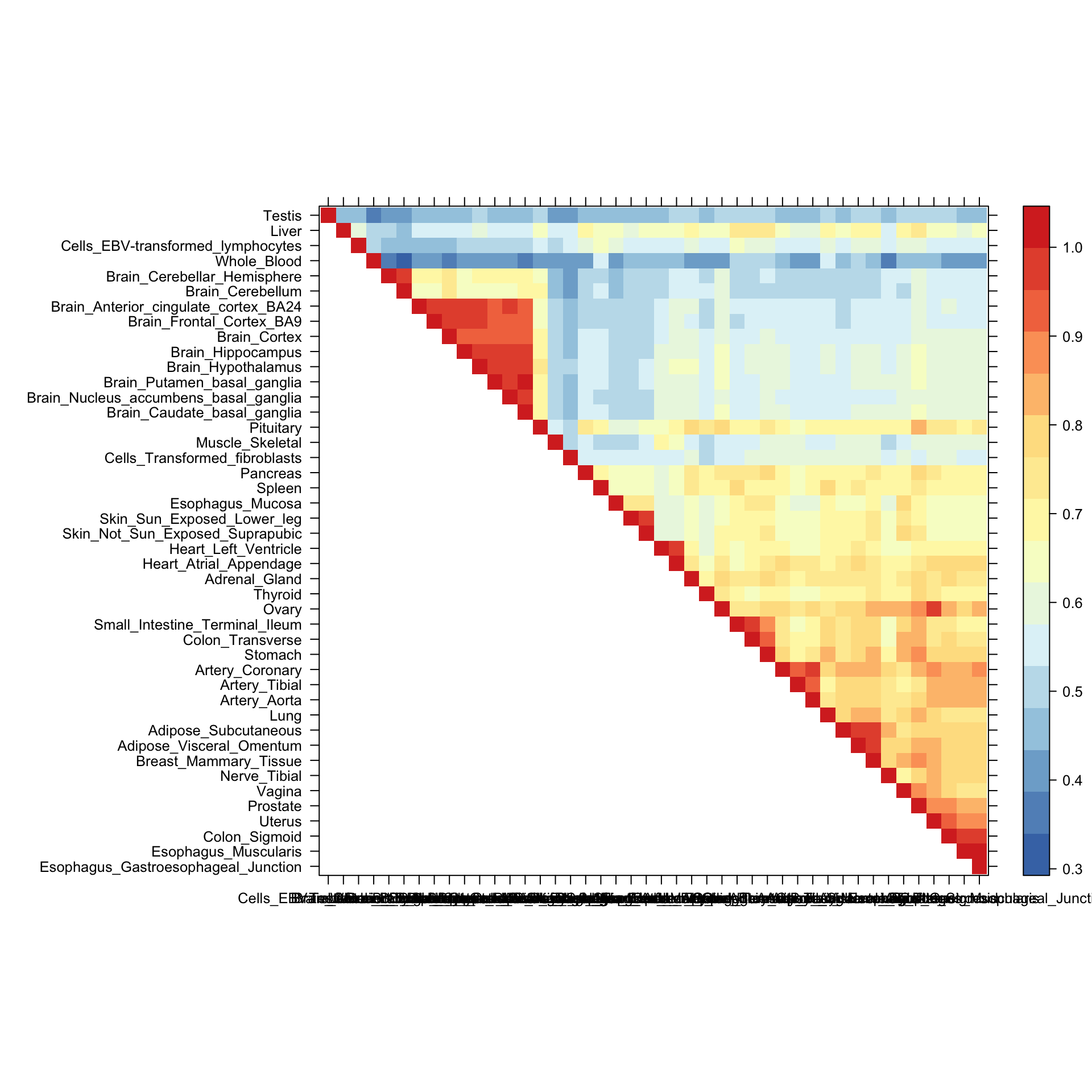
Session information
sessionInfo()
R version 3.4.3 (2017-11-30)
Platform: x86_64-apple-darwin15.6.0 (64-bit)
Running under: macOS High Sierra 10.13.4

Matrix products: default
BLAS: /Library/Frameworks/R.framework/Versions/3.4/Resources/lib/libRblas.0.dylib
LAPACK: /Library/Frameworks/R.framework/Versions/3.4/Resources/lib/libRlapack.dylib

locale:
[1] en_US.UTF-8/en_US.UTF-8/en_US.UTF-8/C/en_US.UTF-8/en_US.UTF-8

attached base packages:
[1] stats     graphics  grDevices utils     datasets  methods   base

other attached packages:
[1] lattice_0.20-35

loaded via a namespace (and not attached):
 [1] workflowr_1.0.1.9000 Rcpp_0.12.16         digest_0.6.15
 [4] rprojroot_1.3-2      R.methodsS3_1.7.1    grid_3.4.3
 [7] backports_1.1.2      git2r_0.21.0         magrittr_1.5
[10] evaluate_0.10.1      stringi_1.1.7        whisker_0.3-2
[13] R.oo_1.21.0          R.utils_2.6.0        rmarkdown_1.9
[16] tools_3.4.3          stringr_1.3.0        yaml_2.1.18
[19] compiler_3.4.3       htmltools_0.3.6      knitr_1.20
This reproducible R Markdown analysis was created with workflowr 1.0.1.9000