Primary correlation patterns identified by mash in GTEx data
Sarah Urbut, Gao Wang, Peter Carbonetto and Matthew Stephens
Last updated: 2018-06-05
workflowr checks: (Click a bullet for more information)-
✔ R Markdown file: up-to-date
Great! Since the R Markdown file has been committed to the Git repository, you know the exact version of the code that produced these results.
-
✔ Environment: empty
Great job! The global environment was empty. Objects defined in the global environment can affect the analysis in your R Markdown file in unknown ways. For reproduciblity it’s best to always run the code in an empty environment.
-
✔ Seed:
set.seed(1)The command
set.seed(1)was run prior to running the code in the R Markdown file. Setting a seed ensures that any results that rely on randomness, e.g. subsampling or permutations, are reproducible. -
✔ Session information: recorded
Great job! Recording the operating system, R version, and package versions is critical for reproducibility.
-
Great! You are using Git for version control. Tracking code development and connecting the code version to the results is critical for reproducibility. The version displayed above was the version of the Git repository at the time these results were generated.✔ Repository version: a9bca8b
Note that you need to be careful to ensure that all relevant files for the analysis have been committed to Git prior to generating the results (you can usewflow_publishorwflow_git_commit). workflowr only checks the R Markdown file, but you know if there are other scripts or data files that it depends on. Below is the status of the Git repository when the results were generated:
Note that any generated files, e.g. HTML, png, CSS, etc., are not included in this status report because it is ok for generated content to have uncommitted changes.Ignored files: Ignored: .sos/ Ignored: data/.sos/ Ignored: output/MatrixEQTLSumStats.Portable.Z.coved.K3.P3.lite.single.expanded.V1.loglik.rds Ignored: workflows/.ipynb_checkpoints/ Ignored: workflows/.sos/ Untracked files: Untracked: TODO.txt Untracked: analysis/files.txt Untracked: fastqtl_to_mash_output/ Untracked: gtex6_workflow_output/ Unstaged changes: Deleted: analysis/Fig.Uk2.Rmd Deleted: analysis/Fig.Uk3.Rmd Deleted: analysis/Fig.Uk4.Rmd Deleted: analysis/Fig.Uk5.Rmd Deleted: analysis/Fig.Uk8.Rmd Modified: analysis/gtex.Rmd
Expand here to see past versions:
“Uk3” is the covariance matrix corresponding to the output of the ExtremeDeconvolution algorithm that was initialized with the rank3 SVD approximation of \(X^TX\). It is the pattern of sharing identified from the dominant covariance matrix (the one with the largest mixture weight).
Here we plot the correlation matrix and the first 3 eigenvectors of “Uk3”. This provides a visualization of the primary patterns of genetic sharing identified by our method, mash. This code should closely reproduce Figure 3 of the paper.
Set up environment
First, we load a couple plotting packages used in the code chunks below.
library(lattice)
library(colorRamps)
Load data and mash results
We load some GTEx summary statistics, as well as some of the results generated from the mash analysis of the GTEx data.
covmat <- readRDS(paste("../output/MatrixEQTLSumStats.Portable.Z.coved.K3.P3",
                        "lite.single.expanded.rds",sep = "."))
pis    <- readRDS(paste("../output/MatrixEQTLSumStats.Portable.Z.coved.K3.P3",
                        "lite.single.expanded.V1.pihat.rds",sep = "."))$pihat
z.stat <- readRDS("../data/MatrixEQTLSumStats.Portable.Z.rds")$test.z
pi.mat <- matrix(pis[-length(pis)],ncol = 54,nrow = 22,byrow = TRUE)
names  <- colnames(z.stat)
colnames(pi.mat) <-
  c("ID","X'X","SVD","F1","F2","F3","F4","F5","SFA_Rank5",names,"ALL")
Compute the correlations from the \(k=3\) covariance matrix.
k        <- 3
x        <- cov2cor(covmat[[k]])
x[x < 0] <- 0
Next, we load the tissue indices and tissue names:
colnames(x) <- names
rownames(x) <- names
h <- read.table("../data/uk3rowindices.txt")[,1]
For the plots of the eigenvectors, we load the colours that are conventionally used to represent the tissues in plots.
missing.tissues <- c(7,8,19,20,24,25,31,34,37)
color.gtex <- read.table("../data/GTExColors.txt",sep = "\t",
                         comment.char = '')[-missing.tissues,]
Summarize relative importance of the covariance matrices
The posterior mixture weights give the relative importance of the covariance matrices for capturing patterns in the data.
barplot(colSums(pi.mat),las = 2,cex.names = 0.5)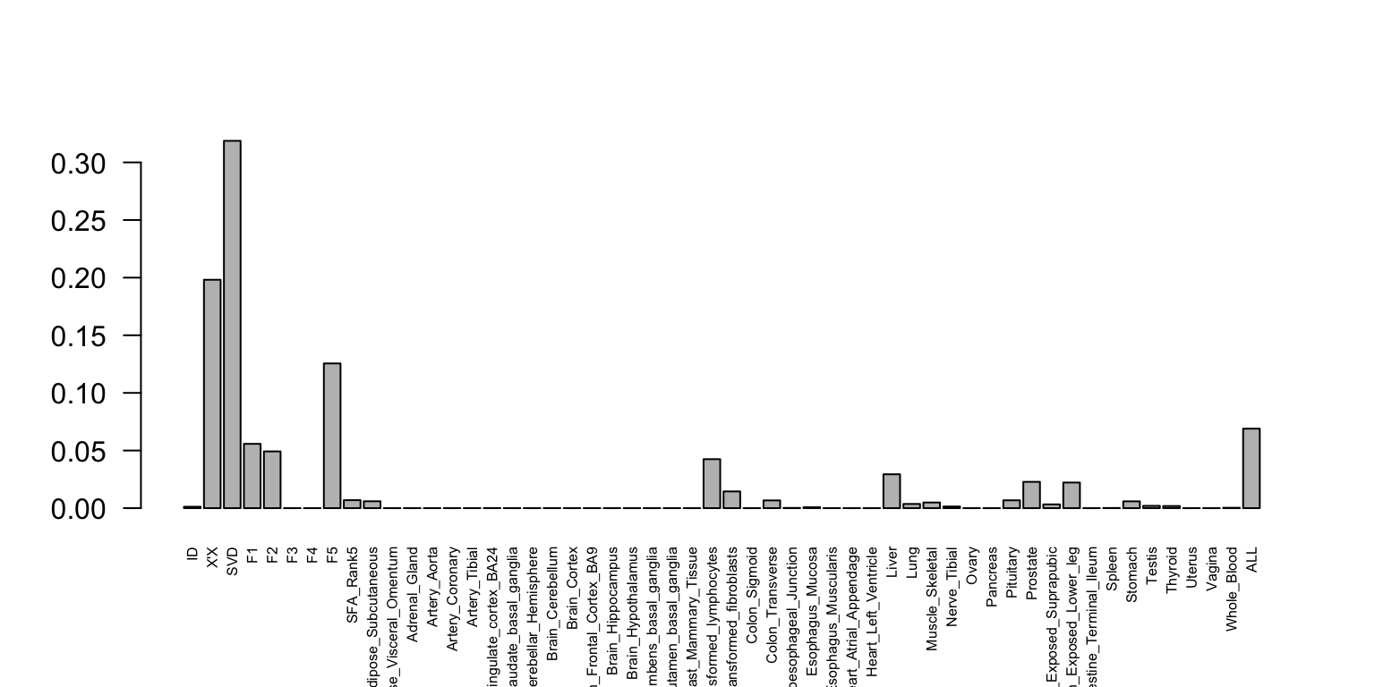
Here we see that the SVD component has the largest weight.
Generate heatmap of Uk3 covariance matrix
Now we produce the heatmap showing the full covariance matrix.
smat <- (x[(h),(h)])
smat[lower.tri(smat)] <- NA
clrs <- colorRampPalette(rev(c("#D73027","#FC8D59","#FEE090","#FFFFBF",
                               "#E0F3F8","#91BFDB","#4575B4")))(64)
lat <- x[rev(h),rev(h)]
lat[lower.tri(lat)] <- NA
n <- nrow(lat)
print(levelplot(lat[n:1,],col.regions = clrs,xlab = "",ylab = "",
                colorkey = TRUE,at = seq(0,1,length.out = 64),
                scales = list(cex = 0.6,x = list(rot = 45))))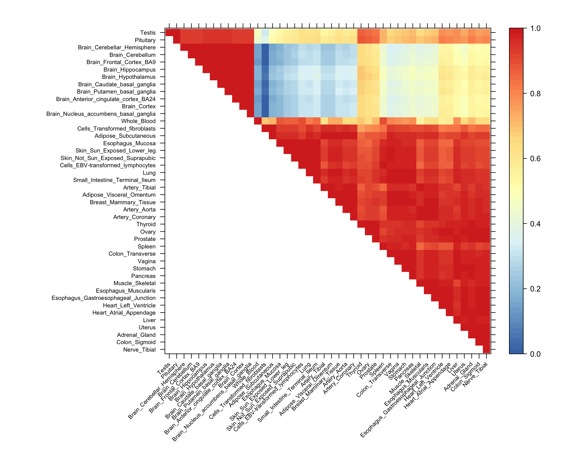
Plot eigenvectors capturing predominant patterns
The eigenvectors capture the predominant patterns in the Uk3 covariance matrix.
k <- 3
vold  <- svd(covmat[[k]])$v
u     <- svd(covmat[[k]])$u
d     <- svd(covmat[[k]])$d
v     <- vold[h,] # Shuffle so correct order
names <- names[h]
color.gtex <- color.gtex[h,]
for (j in 1:3)
  barplot(v[,j]/v[,j][which.max(abs(v[,j]))],names = "",cex.names = 0.5,
          las = 2,main = paste0("EigenVector",j,"Uk",k),
          col = as.character(color.gtex[,2]))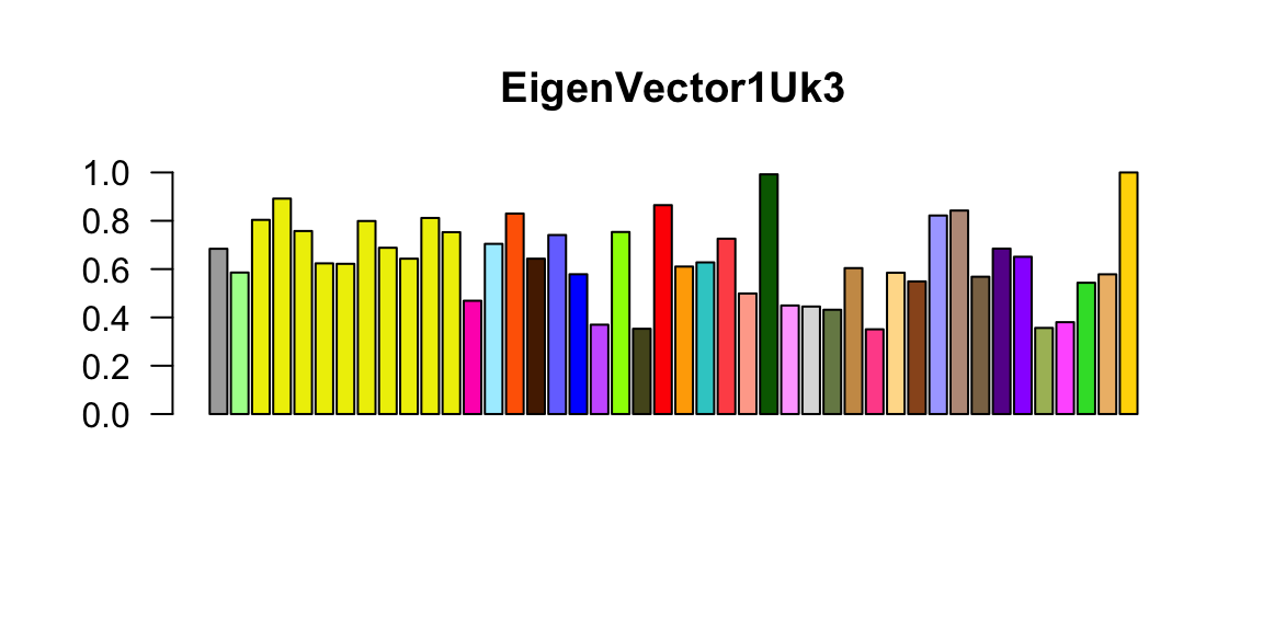
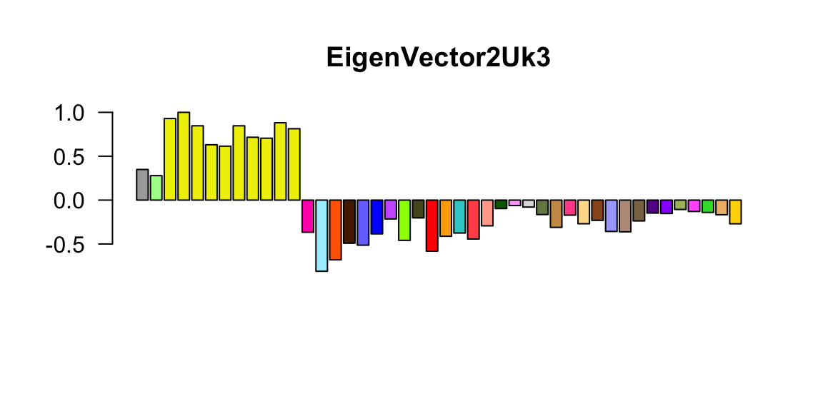
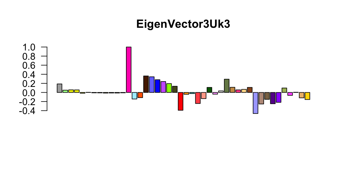
The first eigenvector reflects broad sharing among tissues, with all effects in the same direction; the second eigenvector captures differences between brain (and, to a less extent, testis and pituitary) vs other tissues; the third eigenvector primarily captures effects that are stronger in whole blood than elsewhere.
Session information
sessionInfo()
# R version 3.4.3 (2017-11-30)
# Platform: x86_64-apple-darwin15.6.0 (64-bit)
# Running under: macOS High Sierra 10.13.4
#
# Matrix products: default
# BLAS: /Library/Frameworks/R.framework/Versions/3.4/Resources/lib/libRblas.0.dylib
# LAPACK: /Library/Frameworks/R.framework/Versions/3.4/Resources/lib/libRlapack.dylib
#
# locale:
# [1] en_US.UTF-8/en_US.UTF-8/en_US.UTF-8/C/en_US.UTF-8/en_US.UTF-8
#
# attached base packages:
# [1] stats     graphics  grDevices utils     datasets  methods   base
#
# other attached packages:
# [1] colorRamps_2.3  lattice_0.20-35
#
# loaded via a namespace (and not attached):
#  [1] workflowr_1.0.1.9000 Rcpp_0.12.16         digest_0.6.15
#  [4] rprojroot_1.3-2      R.methodsS3_1.7.1    grid_3.4.3
#  [7] backports_1.1.2      git2r_0.21.0         magrittr_1.5
# [10] evaluate_0.10.1      stringi_1.1.7        whisker_0.3-2
# [13] R.oo_1.21.0          R.utils_2.6.0        rmarkdown_1.9
# [16] tools_3.4.3          stringr_1.3.0        yaml_2.1.18
# [19] compiler_3.4.3       htmltools_0.3.6      knitr_1.20
This reproducible R Markdown analysis was created with workflowr 1.0.1.9000