l0learn_challenge
stephens999
2018-12-08
Last updated: 2018-12-14
workflowr checks: (Click a bullet for more information)-
✔ R Markdown file: up-to-date
Great! Since the R Markdown file has been committed to the Git repository, you know the exact version of the code that produced these results.
-
✔ Environment: empty
Great job! The global environment was empty. Objects defined in the global environment can affect the analysis in your R Markdown file in unknown ways. For reproduciblity it’s best to always run the code in an empty environment.
-
✔ Seed:
set.seed(20180414)The command
set.seed(20180414)was run prior to running the code in the R Markdown file. Setting a seed ensures that any results that rely on randomness, e.g. subsampling or permutations, are reproducible. -
✔ Session information: recorded
Great job! Recording the operating system, R version, and package versions is critical for reproducibility.
-
Great! You are using Git for version control. Tracking code development and connecting the code version to the results is critical for reproducibility. The version displayed above was the version of the Git repository at the time these results were generated.✔ Repository version: ba91480
Note that you need to be careful to ensure that all relevant files for the analysis have been committed to Git prior to generating the results (you can usewflow_publishorwflow_git_commit). workflowr only checks the R Markdown file, but you know if there are other scripts or data files that it depends on. Below is the status of the Git repository when the results were generated:
Note that any generated files, e.g. HTML, png, CSS, etc., are not included in this status report because it is ok for generated content to have uncommitted changes.Ignored files: Ignored: .DS_Store Ignored: .Rhistory Ignored: .Rproj.user/ Ignored: analysis/.Rhistory Ignored: docs/.DS_Store Ignored: docs/figure/.DS_Store Untracked files: Untracked: analysis/cp_init_locs.Rmd Untracked: analysis/null.Rmd Untracked: analysis/test.Rmd Untracked: data/geneMatrix.tsv Untracked: data/liter_data_4_summarize_ld_1_lm_less_3.rds Untracked: data/meta.tsv Untracked: docs/figure/cp_init_locs.Rmd/ Untracked: docs/figure/test.Rmd/ Untracked: sim_cp.pdf Unstaged changes: Modified: analysis/changepoint.Rmd
Expand here to see past versions:
Introduction
The aim here is to illustrate L0learn’s performance on a challenging example that we also use to challenge susie.
library("L0Learn")
library("genlasso")
Loading required package: MatrixLoading required package: igraph
Attaching package: 'igraph'The following objects are masked from 'package:stats':
decompose, spectrumThe following object is masked from 'package:base':
unionSimple changepoint example
Here we simulate some data with two changepoints, very close together. (Note: a more challenging example still might make these even closer together?)
set.seed(1)
x = rnorm(100)
x[50:51]=x[50:51]+8
plot(x, col="gray")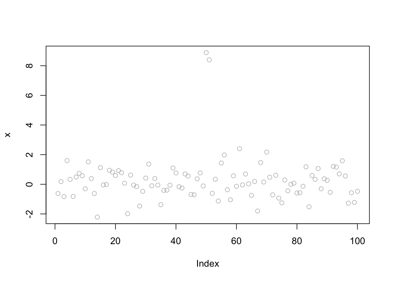
Expand here to see past versions of unnamed-chunk-2-1.png:
| Version | Author | Date |
|---|---|---|
| 4e79e79 | stephens999 | 2018-12-08 |
Now we set up the design matrix \(X\) to use a “step function” basis.
n = length(x)
X = matrix(0,nrow=n,ncol=n-1)
for(j in 1:(n-1)){
  for(i in (j+1):n){
    X[i,j] = 1
  }
}
Now try L0Learn with L0 penalty. (Note: The CD algorithm is the faster and less accurate one.)
y.l0.CD = L0Learn.fit(X,x,penalty="L0",maxSuppSize = 100,autoLambda = FALSE,lambdaGrid = list(seq(0.01,0.001,length=100)),algorithm="CD")


y.l0.CDPSI = L0Learn.fit(X,x,penalty="L0",maxSuppSize = 100,autoLambda = FALSE,lambdaGrid = list(seq(0.0076,0.0075,length=1000)),algorithm="CDPSI")

plot(x,main="green=CDPSI; red=CD")
lines(predict(y.l0.CD,newx=X,lambda=y.l0.CD$lambda[[1]][min(which(y.l0.CD$suppSize[[1]]>1))]),col=2)
lines(predict(y.l0.CDPSI,newx=X,lambda=y.l0.CDPSI$lambda[[1]][min(which(y.l0.CDPSI$suppSize[[1]]>1))]),col=3)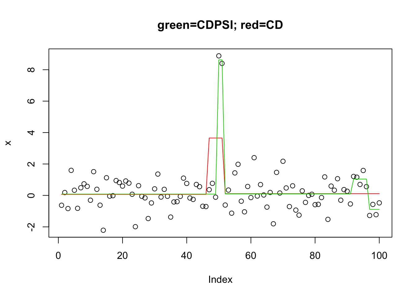
Expand here to see past versions of unnamed-chunk-4-1.png:
| Version | Author | Date |
|---|---|---|
| 4e79e79 | stephens999 | 2018-12-08 |
head(y.l0.CD$suppSize[[1]])[1] 2 2 2 2 2 2head(y.l0.CDPSI$suppSize[[1]])[1] 4 4 4 4 4 4Note that the more sophisticated CSPSI algorithm does not find the correct solution here because it does not give 2 changepoints - all solutions have at least 4 changepoints. I guess it might be possible to solve this by playing with the penalty?
Indeed, Rahul Mazumder sent me this code, which indeed recovers the solution with both algorithms:
y.l0.CD = L0Learn.fit(X,x,penalty="L0",maxSuppSize = 100,autoLambda = FALSE,lambdaGrid = list(seq(0.001,1,length=100)),
                      algorithm="CD")

y.l0.CDPSI = L0Learn.fit(X,x,penalty="L0",maxSuppSize = 100,autoLambda = FALSE,lambdaGrid = list(seq(0.001,1,length=100)),algorithm="CDPSI")

plot(x,main="green=CDPSI; red=CD")
lines(predict(y.l0.CD, newx=X, lambda=y.l0.CD$lambda[[1]][50]),col=2) #
lines(predict(y.l0.CDPSI, newx=X, lambda=y.l0.CDPSI$lambda[[1]][50]),col=3) 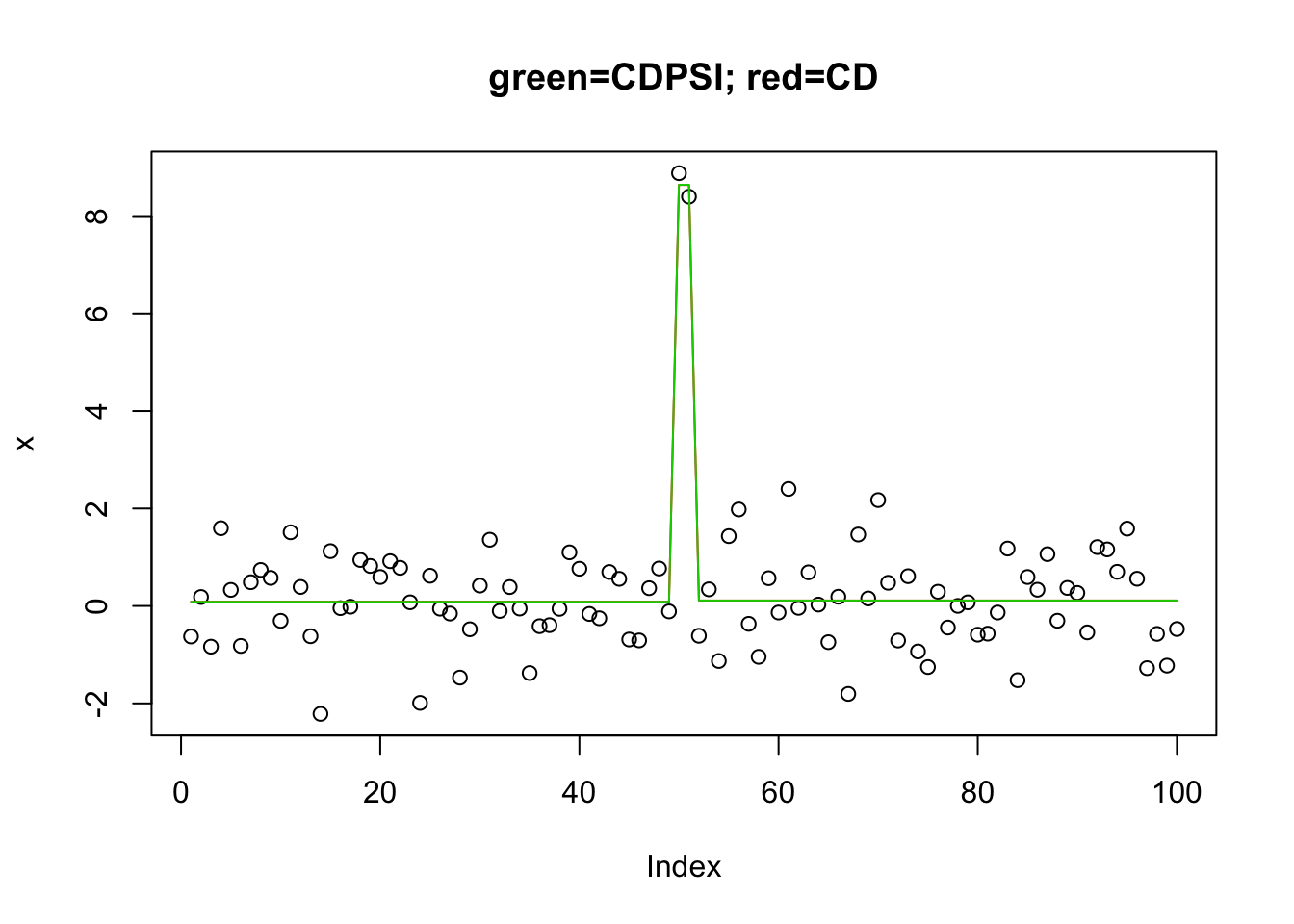
I found it interesting that this did not work when I reversed the lambda. I guess this is maybe analogous to the difference between “backwards” vs “forwards” selection?
y.l0.CD = L0Learn.fit(X,x,penalty="L0",maxSuppSize = 100,autoLambda = FALSE,lambdaGrid = list(seq(1,0.001,length=100)),
                      algorithm="CD")

y.l0.CDPSI = L0Learn.fit(X,x,penalty="L0",maxSuppSize = 100,autoLambda = FALSE,lambdaGrid = list(seq(1,0.001,length=100)),algorithm="CDPSI")

plot(x,main="green=CDPSI; red=CD")
lines(predict(y.l0.CD, newx=X, lambda=y.l0.CD$lambda[[1]][50]),col=2) # recovers the soln

lines(predict(y.l0.CDPSI, newx=X, lambda=y.l0.CDPSI$lambda[[1]][50]),col=3) #recovers the soln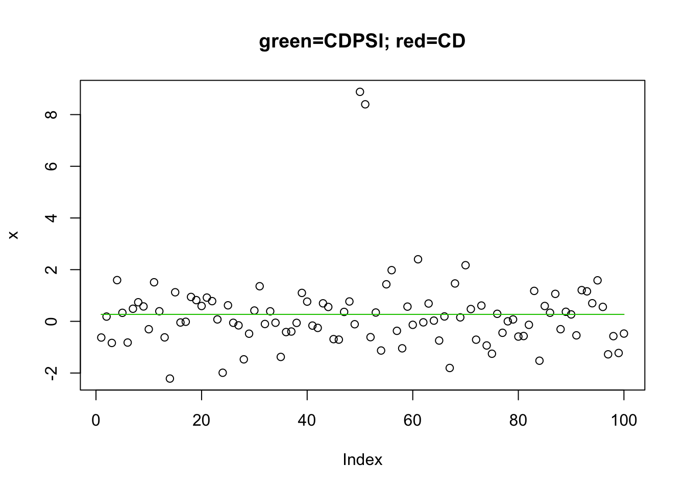
Interestingly(?) the CDPSI does actually recover the correct solution at a different lamdba:
y.l0.CDPSI$suppSize[[1]] [1] 0 0 0 0 0 0 0 0 0 0 0 0 0 0 0 0 0 0 0 0 0 0 0
[24] 0 0 0 0 0 0 0 0 0 0 0 0 0 0 0 0 0 0 0 0 0 0 0
[47] 0 0 0 0 0 0 0 0 0 0 0 0 0 0 0 0 0 0 0 0 0 0 0
[70] 0 0 0 0 0 0 0 0 0 0 0 0 0 0 0 0 0 0 0 0 0 0 0
[93] 0 0 0 0 0 0 2 20y.l0.CDPSI$suppSize[[1]] [1] 0 0 0 0 0 0 0 0 0 0 0 0 0 0 0 0 0 0 0 0 0 0 0
[24] 0 0 0 0 0 0 0 0 0 0 0 0 0 0 0 0 0 0 0 0 0 0 0
[47] 0 0 0 0 0 0 0 0 0 0 0 0 0 0 0 0 0 0 0 0 0 0 0
[70] 0 0 0 0 0 0 0 0 0 0 0 0 0 0 0 0 0 0 0 0 0 0 0
[93] 0 0 0 0 0 0 2 20plot(x,main="green=CDPSI; red=CD")
lines(predict(y.l0.CD, newx=X, lambda=y.l0.CD$lambda[[1]][99]),col=2) # recovers the soln
lines(predict(y.l0.CDPSI, newx=X, lambda=y.l0.CDPSI$lambda[[1]][99]),col=3) #recovers the soln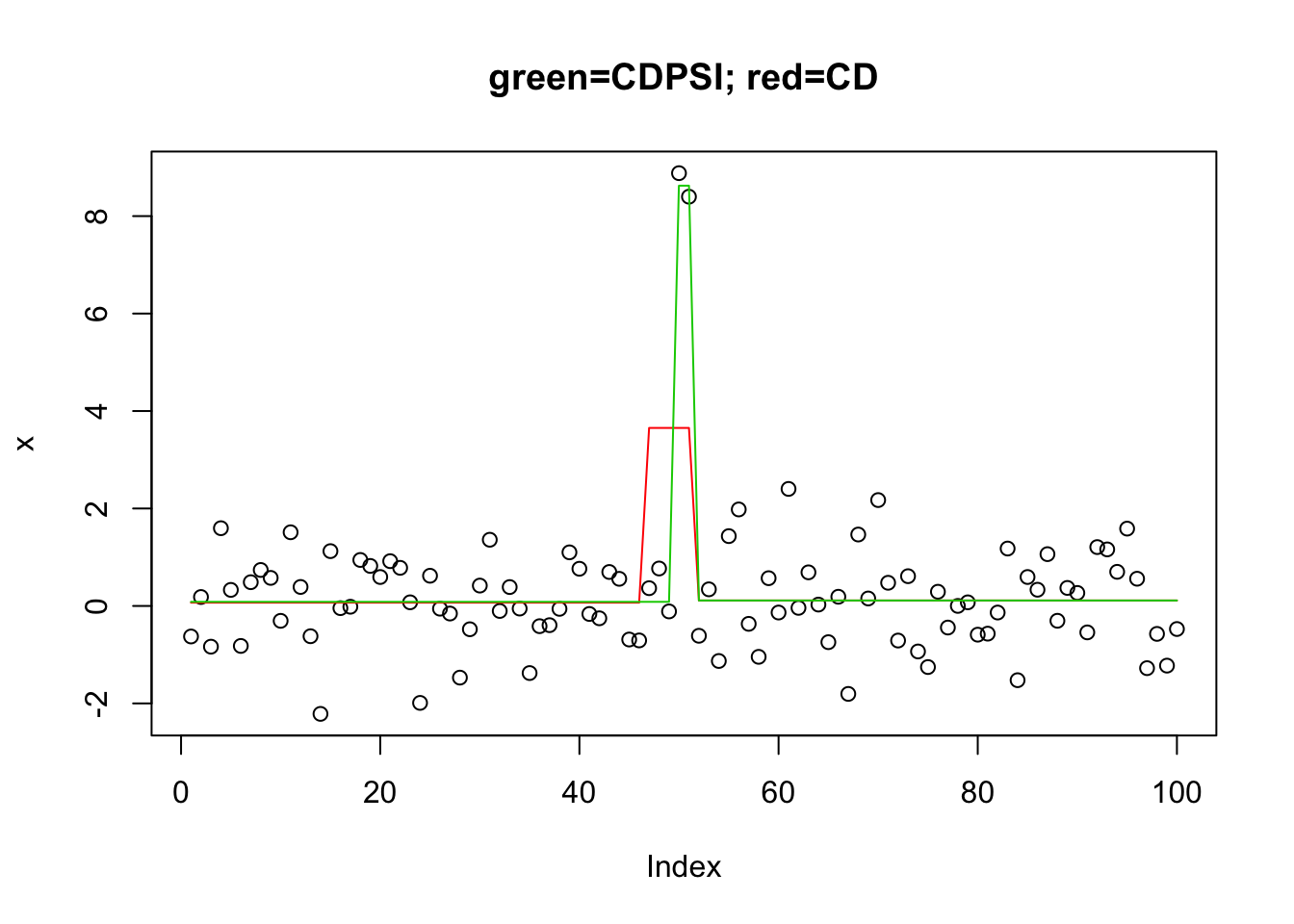
Session information
sessionInfo()R version 3.5.1 (2018-07-02)
Platform: x86_64-apple-darwin15.6.0 (64-bit)
Running under: OS X El Capitan 10.11.6
Matrix products: default
BLAS: /Library/Frameworks/R.framework/Versions/3.5/Resources/lib/libRblas.0.dylib
LAPACK: /Library/Frameworks/R.framework/Versions/3.5/Resources/lib/libRlapack.dylib
locale:
[1] en_US.UTF-8/en_US.UTF-8/en_US.UTF-8/C/en_US.UTF-8/en_US.UTF-8
attached base packages:
[1] stats graphics grDevices utils datasets methods base
other attached packages:
[1] genlasso_1.4 igraph_1.2.2 Matrix_1.2-14 L0Learn_1.0.7
loaded via a namespace (and not attached):
[1] Rcpp_1.0.0 compiler_3.5.1 pillar_1.3.0
[4] git2r_0.23.0 plyr_1.8.4 workflowr_1.1.1
[7] bindr_0.1.1 R.methodsS3_1.7.1 R.utils_2.7.0
[10] tools_3.5.1 digest_0.6.18 evaluate_0.12
[13] tibble_1.4.2 gtable_0.2.0 lattice_0.20-35
[16] pkgconfig_2.0.2 rlang_0.2.2 yaml_2.2.0
[19] bindrcpp_0.2.2 stringr_1.3.1 dplyr_0.7.7
[22] knitr_1.20 tidyselect_0.2.5 rprojroot_1.3-2
[25] grid_3.5.1 glue_1.3.0 R6_2.3.0
[28] rmarkdown_1.10 reshape2_1.4.3 purrr_0.2.5
[31] ggplot2_3.0.0 magrittr_1.5 whisker_0.3-2
[34] backports_1.1.2 scales_1.0.0 htmltools_0.3.6
[37] assertthat_0.2.0 colorspace_1.3-2 stringi_1.2.4
[40] lazyeval_0.2.1 munsell_0.5.0 crayon_1.3.4
[43] R.oo_1.22.0 This reproducible R Markdown analysis was created with workflowr 1.1.1