changepoint

Introduction

Here we try susie on some example change point problems, and compare with other methods for change point detection in the changepoint package (penalized methods), bcp package (Bayesian MCMC method), and genlasso (L1 penalty method).

First we define some useful functions to run susie on changepoint problems and plot the CSs.

susie_cp = function(y,auto=FALSE,...){
  n=length(y)
  X = matrix(0,nrow=n,ncol=n-1)
  for(j in 1:(n-1)){
    for(i in (j+1):n){
      X[i,j] = 1
    }
  }
  if(auto){
    s = susie_auto(X,y,...)
  } else {
    s = susie(X,y,...)
  }
  return(s)
}

#plot a time series y with confidence sets from susie fit s overlaid
# does - 0.5 so that singletons show up
# this is a ggplot version
susie_plot_cp = function(s,y){
  library("ggplot2")
  df<-data.frame(x = 1:length(y),y = y)
  CS = s$sets$cs

  p= ggplot(df) + geom_point(mapping=aes_string(x="x", y="y"))
  for(i in 1:length(CS)){
    p = p + annotate("rect", fill = "red", alpha = 0.5, 
        xmin = min(CS[[i]])-0.5, xmax = max(CS[[i]])+0.5,
        ymin = -Inf, ymax = Inf) 
  }
  p
}

# this is just a function to add the changepoints to a base grapics plot
plot_cs = function(s){
  CS = s$sets$cs
  for(i in 1:length(CS)){
    rect(min(CS[[i]])-0.5,-5,max(CS[[i]])+0.5,5,col = rgb(1,0,0,alpha=0.5),border=NA)
  }
}

Simple simulated example

This example comes from Killick and Eckley

library(changepoint)

Loading required package: zoo

Attaching package: 'zoo'

The following objects are masked from 'package:base':

    as.Date, as.Date.numeric

Successfully loaded changepoint package version 2.2.2
 NOTE: Predefined penalty values changed in version 2.2.  Previous penalty values with a postfix 1 i.e. SIC1 are now without i.e. SIC and previous penalties without a postfix i.e. SIC are now with a postfix 0 i.e. SIC0. See NEWS and help files for further details.

set.seed(10)
eg1=c(rnorm(100,0,1),rnorm(100,1,1),rnorm(100,0,1),rnorm(100,0.2,1)) 
ts.plot(eg1,xlab="Index")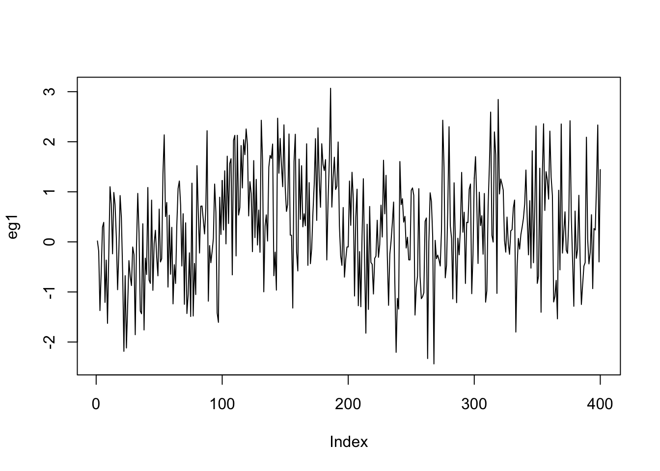

Expand here to see past versions of unnamed-chunk-2-1.png:

Version	Author	Date
a45f3cd	stephens999	2018-10-18

true_mean = c(rep(0,100),rep(1,100),rep(0,100),rep(0.2,100))

Here we apply susie to this example. It finds 2 (out of the three) changepoints.

library("susieR")
eg1.s = susie_cp(eg1)
ts.plot(eg1,xlab="Index")
lines(predict(eg1.s),col=2,lwd=2)
plot_cs(eg1.s)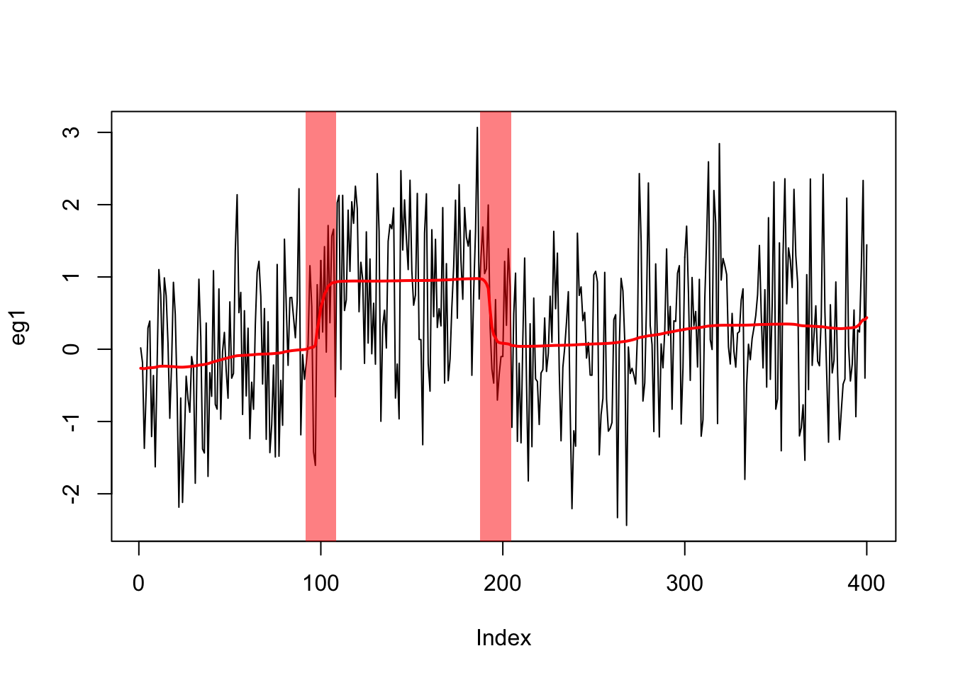

Expand here to see past versions of unnamed-chunk-3-1.png:

Version	Author	Date
a45f3cd	stephens999	2018-10-18

Try the bcp package

library(bcp)

Loading required package: grid

eg1.bcp<- bcp(eg1)
plot(eg1.bcp, main = "Univariate Change Point Example")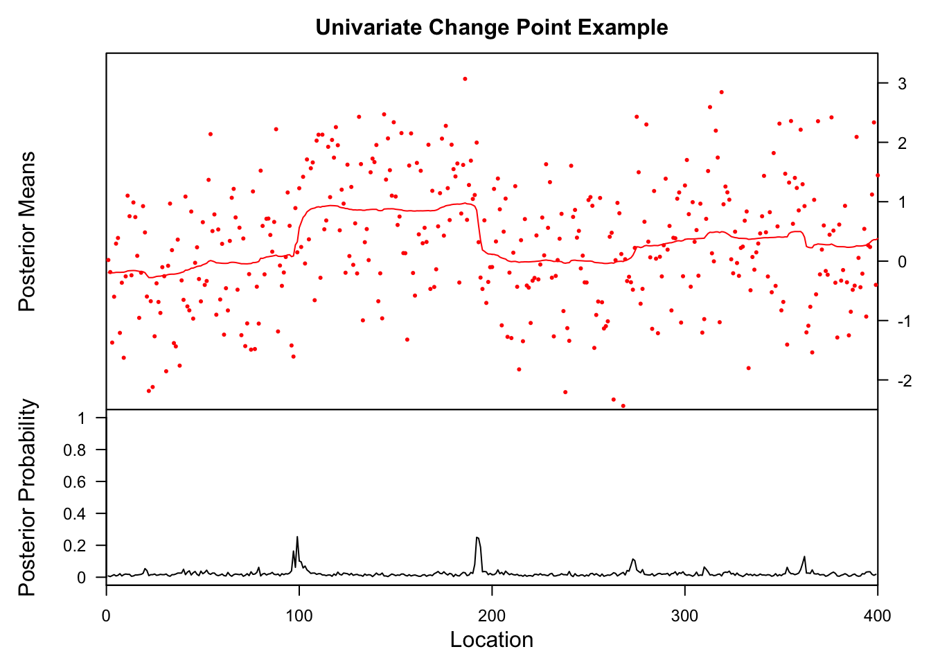

Expand here to see past versions of unnamed-chunk-4-1.png:

Version	Author	Date
a45f3cd	stephens999	2018-10-18

legacyplot(eg1.bcp)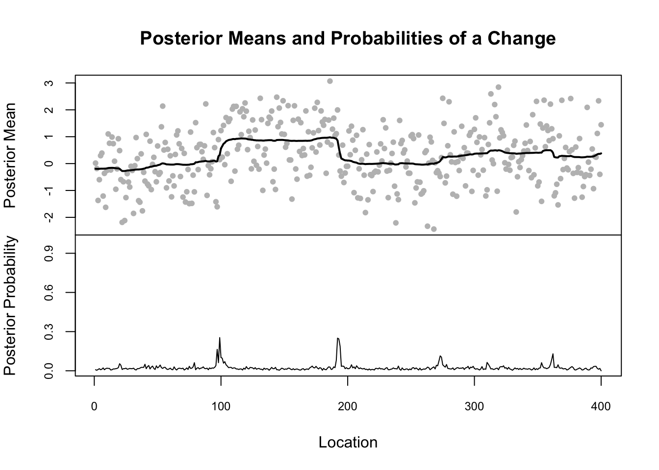

plot(eg1.bcp$posterior.prob[-1], susie_get_PIP(eg1.s))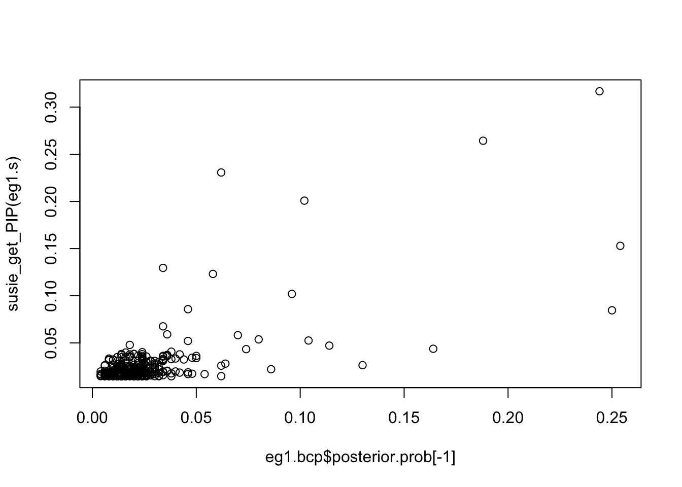

plot(eg1.bcp$posterior.mean, predict(eg1.s))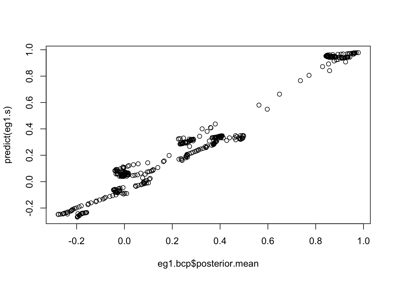

plot(eg1.bcp$posterior.prob[-1])
points(susie_get_PIP(eg1.s), col = 2)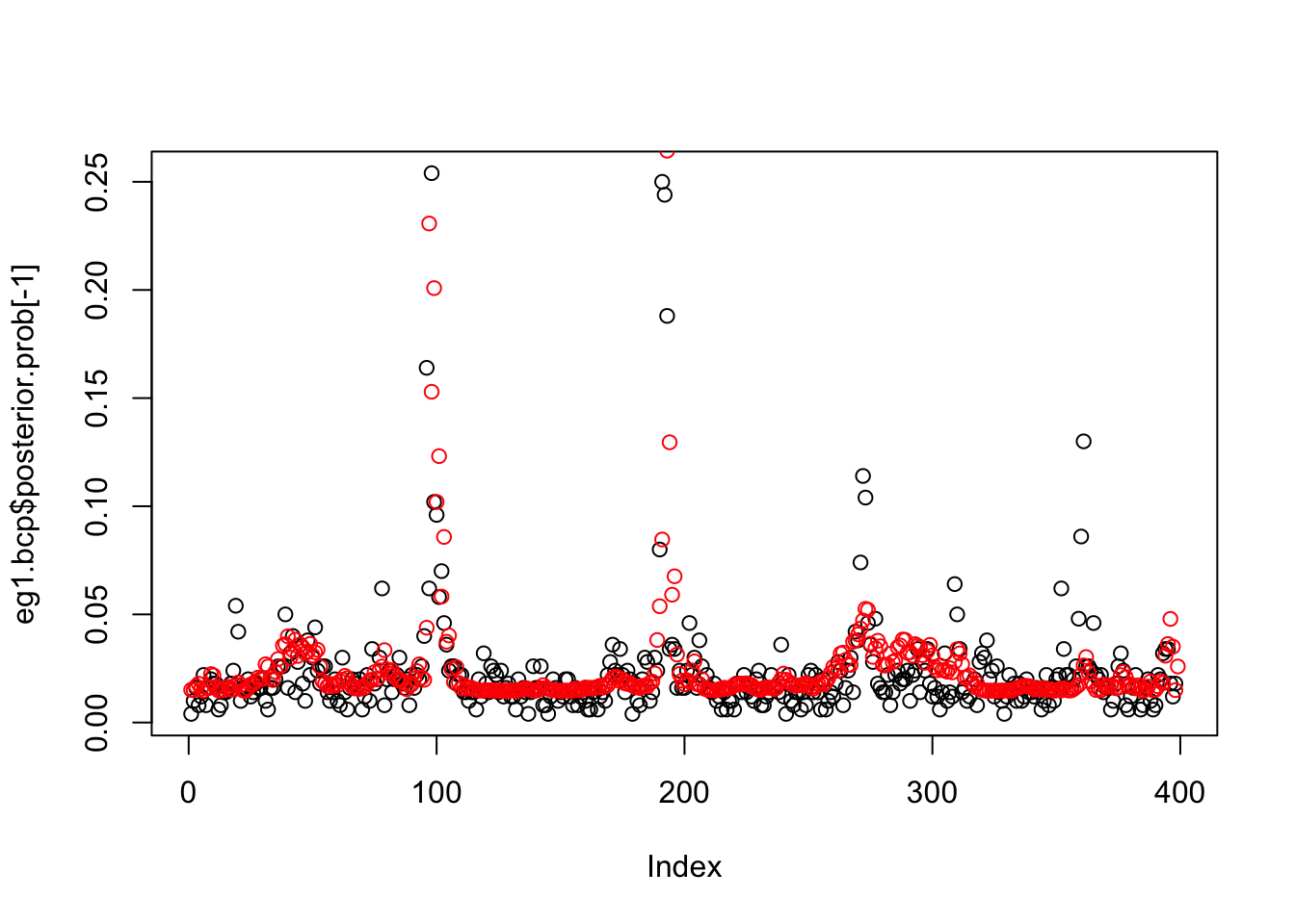

plot(eg1)
lines(true_mean, col = 2, lwd = 2)
lines(predict(eg1.s), col = 3, lwd = 2)
lines(eg1.bcp$posterior.mean, col = 4, lwd = 2)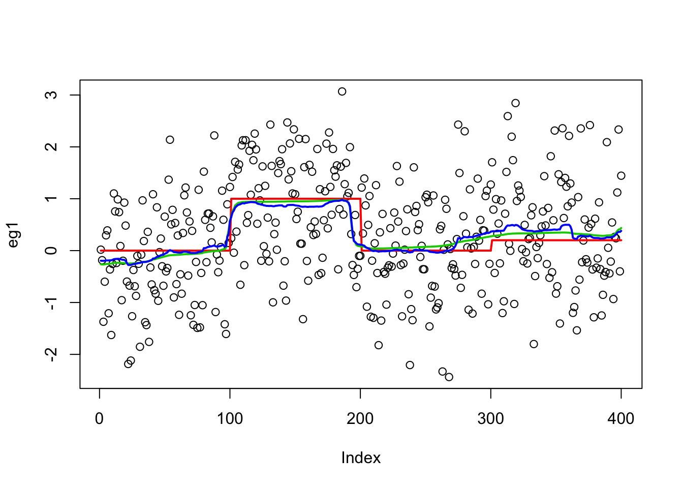

mean((eg1.bcp$posterior.mean - true_mean) ^ 2)

[1] 0.0366996

mean((predict(eg1.s) - true_mean) ^ 2)

[1] 0.03081035

Lai 2005 data

This is a real-data example from the changepoint package.

data(Lai2005fig4)
lai = Lai2005fig4[,5]
lai.default=cpt.mean(lai,method="PELT")
lai.s = susie_cp(lai)
lai.bcp = bcp(lai)
lai.bcp.long = bcp(lai,mcmc=5000)

Results from changepoint:

plot(lai.default,pch=20,col="grey",cpt.col="black",type="p",xlab="Index")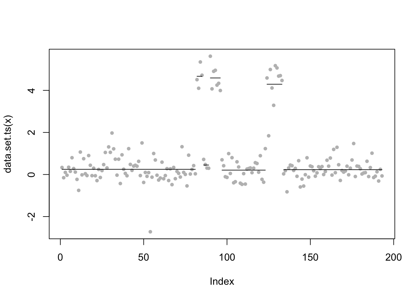 

Expand here to see past versions of unnamed-chunk-6-1.png:

Version	Author	Date
a45f3cd	stephens999	2018-10-18

cpts(lai.default)

[1]  81  85  89  96 123 133

coef(lai.default)

$mean
[1] 0.2468910 4.6699210 0.4495538 4.5902489 0.2079891 4.2913844 0.2291286

From susie (which seems to “miss” one of the changepoints):

plot(lai)
lines(predict(lai.s),col=2)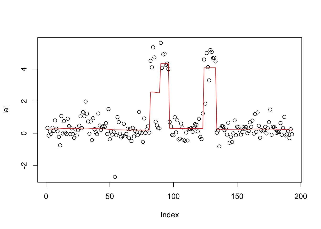

Expand here to see past versions of unnamed-chunk-7-1.png:

Version	Author	Date
a45f3cd	stephens999	2018-10-18

lai.s$elbo

 [1]      -Inf -345.8855 -340.9082 -332.0314 -320.1672 -310.2676 -302.9654
 [8] -297.6058 -293.6073 -290.5957 -288.3099 -286.5210 -284.8860 -282.7483
[15] -280.1089 -278.0768 -276.6409 -275.5822 -274.7859 -274.1864 -273.7356
[22] -273.3947 -273.1329 -272.9270 -272.7608 -272.6239 -272.5094 -272.4130
[29] -272.3319 -272.2641 -272.2079 -272.1621 -272.1250 -272.0952 -272.0716
[36] -272.0529 -272.0381 -272.0265 -272.0175 -272.0105 -272.0051 -272.0010
[43] -271.9979 -271.9955 -271.9938 -271.9925 -271.9915

From bcp:

plot(lai)
lines(lai.bcp$posterior.mean, col = 3, lwd = 2)
lines(lai.bcp.long$posterior.mean, col = 4, lwd = 2)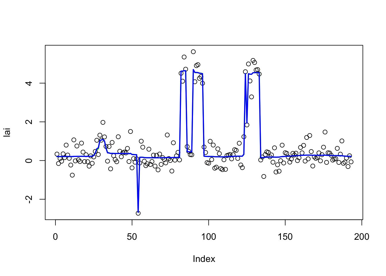

plot(lai.bcp.long$posterior.prob)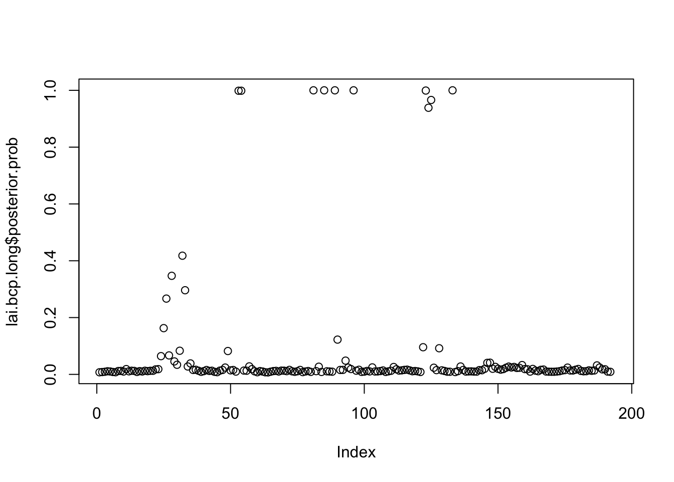

which(lai.bcp.long$posterior.prob>0.99)

[1]  53  54  81  85  89  96 123 133

See if this is maybe a convergence issue solved by susie_auto:

lai.s.auto = susie_cp(lai,auto=TRUE)
plot(lai)
lines(predict(lai.s.auto),col=2)
plot_cs(lai.s.auto)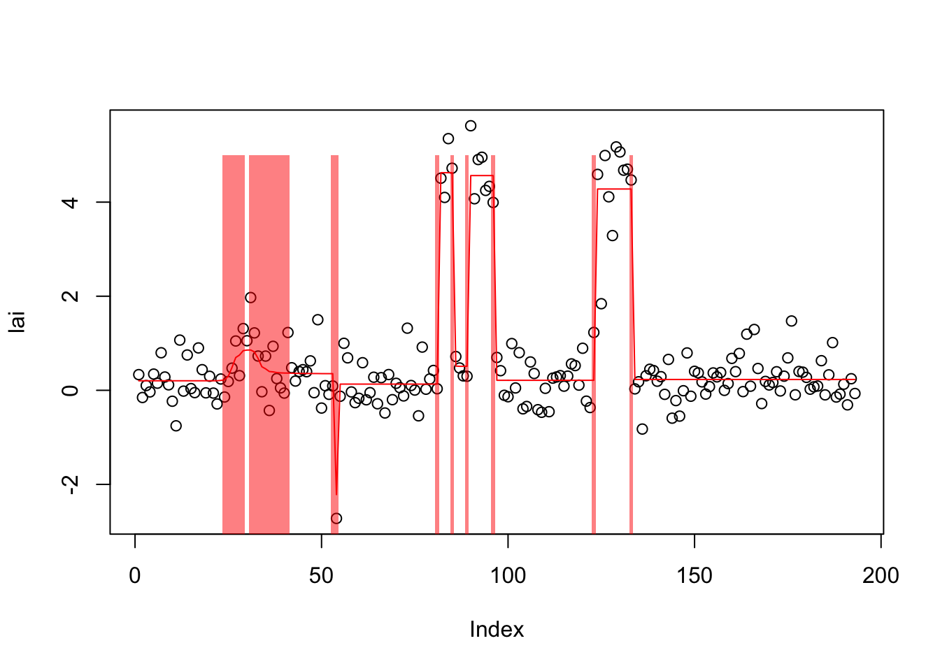

lai.s.auto$elbo

 [1]      -Inf -245.7007 -245.6279 -245.5400 -245.4322 -245.2919 -245.0801
 [8] -244.6691 -243.6458 -242.1472 -241.9562 -241.8816 -241.8067 -241.7264
[15] -241.6426 -241.5578 -241.4743 -241.3936 -241.3169 -241.2447 -241.1771
[22] -241.1140 -241.0552 -241.0004 -240.9494 -240.9017 -240.8572 -240.8154
[29] -240.7762 -240.7393 -240.7045 -240.6717 -240.6407 -240.6114 -240.5836
[36] -240.5572 -240.5322 -240.5084 -240.4858 -240.4643 -240.4439 -240.4244
[43] -240.4059 -240.3882 -240.3714 -240.3554 -240.3401 -240.3255 -240.3116
[50] -240.2984 -240.2858 -240.2737 -240.2622 -240.2513 -240.2408 -240.2309

I wonder if this is an example where the auto version is also finding a local optimum (with many changepoints), and that the best solution would have fewer? Maybe investigate further later.

s0 = susie_init_coef(cpts(lai.default),diff(unlist(coef(lai.default))),length(lai)-1)
lai.s_b = susie_cp(lai,s_init=s0)
plot(lai)
lines(predict(lai.s_b),col=2)
plot_cs(lai.s_b)
lai.s_b$elbo

 [1]      -Inf -476.7494 -429.8976 -383.4484 -348.1532 -320.5661 -302.5209
 [8] -289.8122 -280.1721 -272.7621 -267.0347 -262.5531 -258.9807 -256.0733
[15] -253.6597 -251.6212 -249.8752 -248.3625 -247.0400 -245.8753 -244.8437
[22] -243.9256 -243.1053 -242.3700 -241.7091 -241.1139 -240.5767 -240.0911
[29] -239.6517 -239.2535 -238.8925 -238.5649 -238.2676 -237.9977 -237.7527
[36] -237.5303 -237.3285 -237.1456 -236.9799 -236.8299 -236.6943 -236.5718
[43] -236.4613 -236.3618 -236.2722 -236.1918 -236.1197 -236.0551 -235.9974
[50] -235.9458 -235.8999 -235.8590 -235.8227 -235.7905 -235.7620 -235.7367
[57] -235.7145 -235.6948 -235.6775 -235.6623 -235.6490 -235.6372 -235.6270
[64] -235.6180 -235.6102 -235.6034 -235.5974 -235.5922 -235.5877 -235.5838
[71] -235.5804 -235.5775 -235.5749 -235.5727 -235.5708 -235.5692 -235.5678
[78] -235.5665 -235.5655 -235.5646

lai.s_c = susie_cp(lai,s_init=lai.s_b,estimate_prior_variance=TRUE)
plot_cs(lai.s_c)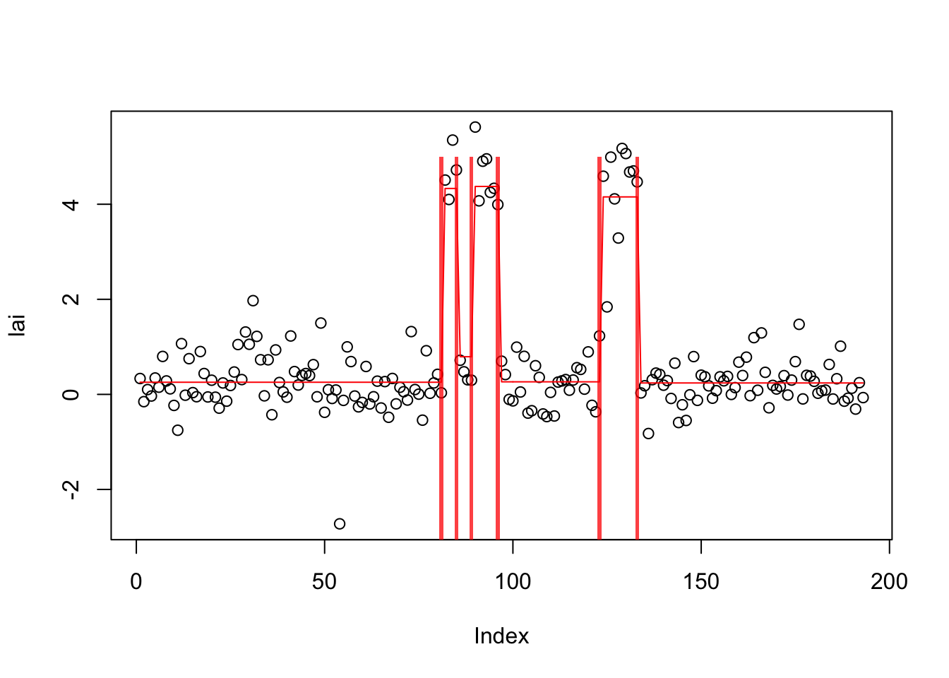

plot(lai)
lines(predict(lai.s_b),col=2,type="s")
plot_cs(lai.s_c)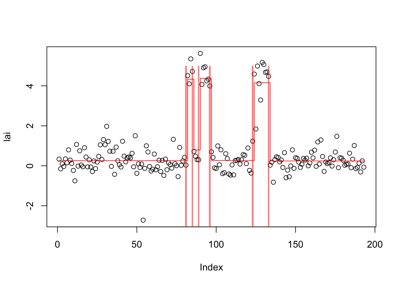

lai.s_c$elbo

 [1]      -Inf -218.6124 -218.3783 -218.1978 -218.0523 -217.9320 -217.8306
 [8] -217.7436 -217.6682 -217.6019 -217.5433 -217.4910 -217.4441 -217.4019
[15] -217.3637 -217.3290 -217.2975 -217.2688 -217.2425 -217.2185 -217.1965
[22] -217.1763 -217.1578 -217.1408 -217.1252 -217.1108 -217.0976 -217.0855
[29] -217.0744 -217.0642 -217.0548 -217.0462 -217.0383 -217.0311 -217.0245
[36] -217.0184 -217.0129 -217.0079 -217.0033 -216.9991 -216.9953 -216.9919
[43] -216.9888 -216.9859 -216.9834 -216.9811 -216.9790 -216.9771 -216.9754
[50] -216.9739 -216.9725 -216.9713 -216.9702 -216.9692

Also try trendfilter in the genlasso package:

library("genlasso")

Loading required package: Matrix

Loading required package: igraph

Attaching package: 'igraph'

The following objects are masked from 'package:stats':

    decompose, spectrum

The following object is masked from 'package:base':

    union

lai.tf = trendfilter(lai,ord=0)
lai.tf.cv = cv.trendfilter(lai.tf)

Fold 1 ... Fold 2 ... Fold 3 ... Fold 4 ... Fold 5 ... 

opt = which(lai.tf$lambda==lai.tf.cv$lambda.min) #optimal value of lambda
lai.tf.fit= lai.tf$fit[,opt]
plot(lai)
lines(lai.tf.fit,type="s",col=2,lwd=2)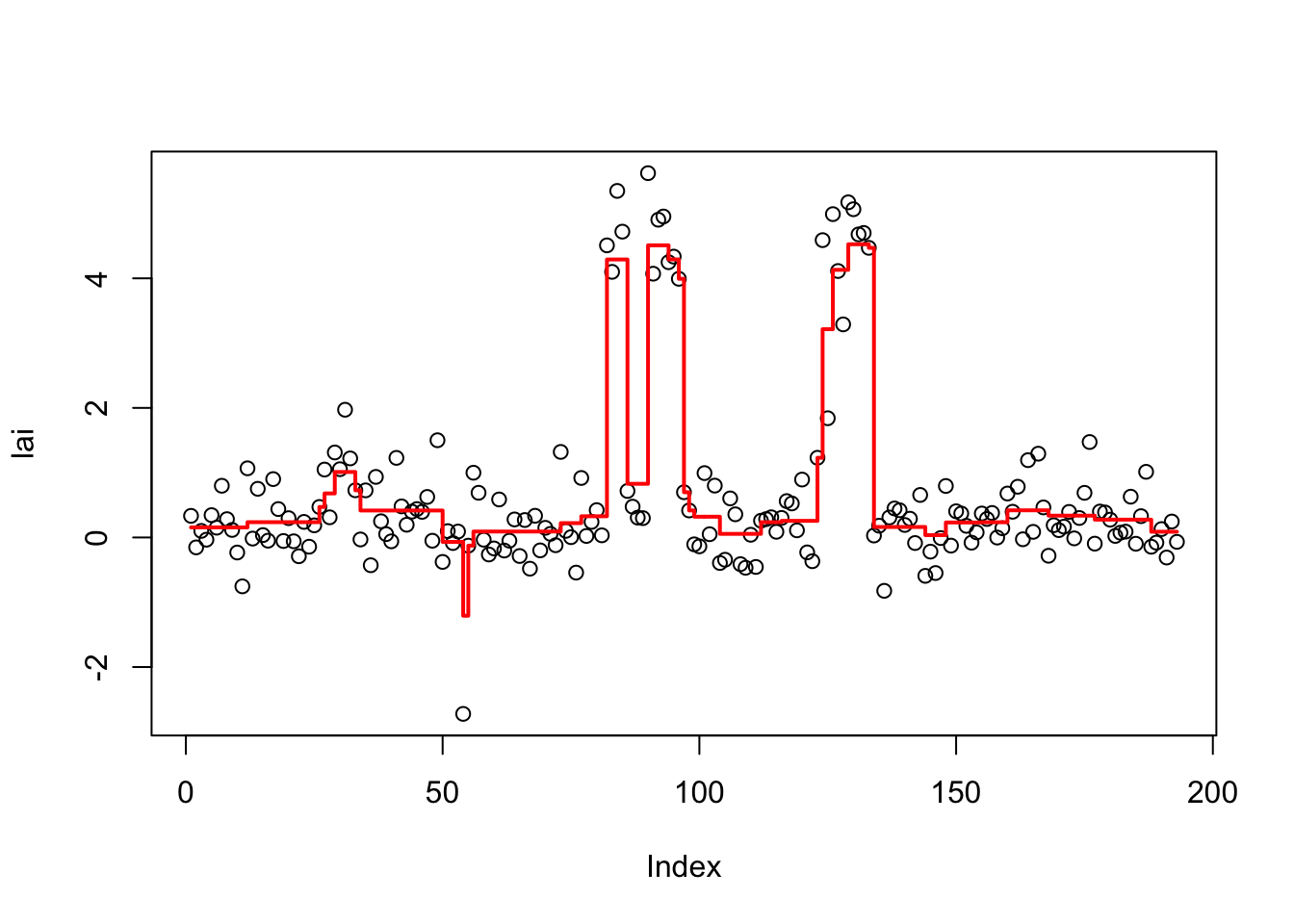

bhat.tf = diff(lai.tf$beta[,opt])
bhat.tf = ifelse(abs(bhat.tf<1e-5),0,bhat.tf) # make very small values 0
s0.tf = susie_init_coef(which(bhat.tf!=0),bhat.tf[bhat.tf!=0],length(lai)-1)
lai.s.tf = susie_cp(lai,s_init = s0.tf,estimate_prior_variance=TRUE)
lai.s.tf$elbo

  [1]      -Inf -405.7173 -364.7052 -344.1847 -336.1369 -332.8231 -330.8278
  [8] -329.1923 -327.5745 -325.1110 -321.0096 -317.6677 -314.5475 -311.6704
 [15] -309.0480 -306.6274 -304.3418 -302.1151 -299.8204 -297.0738 -294.4913
 [22] -293.2757 -292.1828 -291.1844 -290.2599 -289.4007 -288.6002 -287.8530
 [29] -287.1544 -286.5004 -285.8875 -285.3124 -284.7726 -284.2654 -283.7886
 [36] -283.3401 -282.9180 -282.5206 -282.1462 -281.7934 -281.4606 -281.1466
 [43] -280.8500 -280.5696 -280.3043 -280.0528 -279.8140 -279.5866 -279.3695
 [50] -279.1612 -278.9602 -278.7643 -278.5711 -278.3770 -278.1768 -277.9625
 [57] -277.7224 -277.4390 -277.0883 -276.6390 -276.0364 -275.1461 -273.9363
 [64] -272.7732 -272.0091 -271.6603 -271.3907 -271.1490 -270.9279 -270.7239
 [71] -270.5347 -270.3586 -270.1942 -270.0405 -269.8966 -269.7618 -269.6354
 [78] -269.5169 -269.4057 -269.3014 -269.2035 -269.1117 -269.0255 -268.9447
 [85] -268.8688 -268.7976 -268.7307 -268.6679 -268.6089 -268.5535 -268.5014
 [92] -268.4524 -268.4063 -268.3629 -268.3220 -268.2834 -268.2469 -268.2125
 [99] -268.1799 -268.1490 -268.1198

plot(lai)
lines(predict(lai.s.tf),col=2)
plot_cs(lai.s.tf)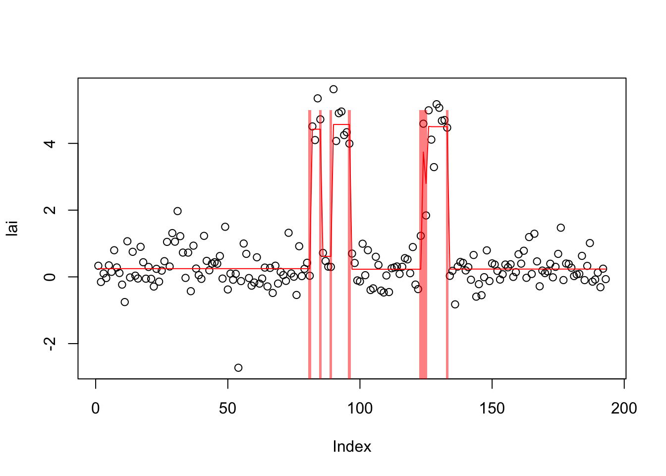

Example from the BCP package

This one is described as a “hard” example (with one change point) in the bcp examples.

set.seed(5)
x <- rep(c(0,1), each=50)
eg2 <- x +  rnorm(50, sd=1)
eg2.bcp <- bcp(eg2)
plot(eg2.bcp, main="Univariate Change Point Example")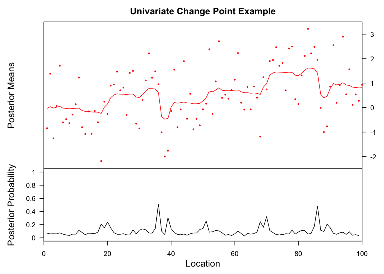

Try susie:

eg2.s = susie_cp(eg2)
plot(eg2)
lines(x,lwd=2)
lines(predict(eg2.s),col=2,lwd=2)
lines(eg2.bcp$posterior.mean,col=3,lwd=2)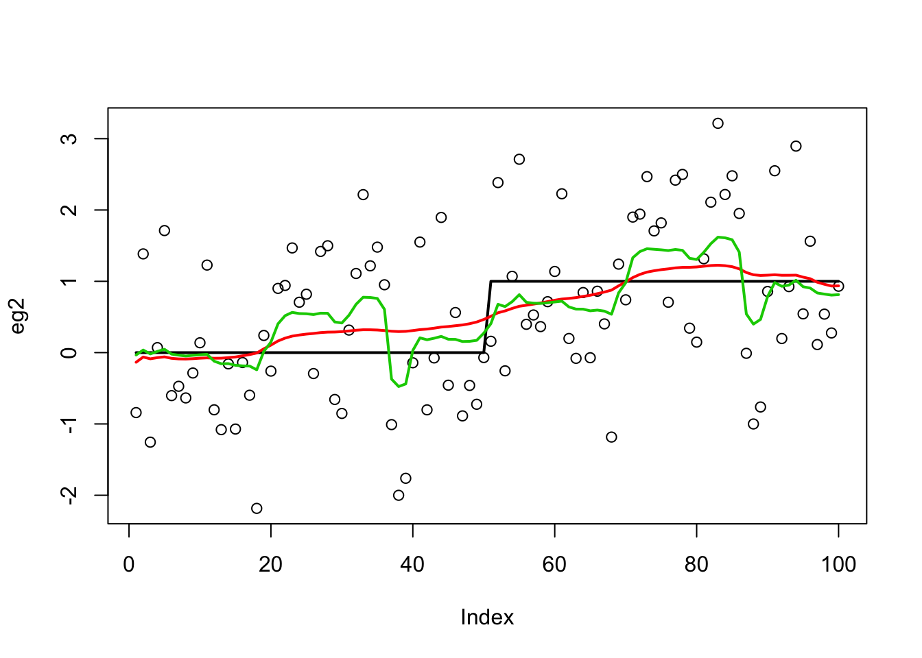

It is a bit wiggly, so try increasing the number of iterations (from default of 500):

eg2.bcp.long <- bcp(eg2,mcmc = 5000,return.mcmc=TRUE)
plot(eg2)
lines(x,lwd=2)
lines(predict(eg2.s),col=2,lwd=2)
lines(eg2.bcp.long$posterior.mean,col=3,lwd=2)
points(eg2.bcp.long$mcmc.means[1000,],col=4,lwd=2)
points(eg2.bcp.long$mcmc.means[5000,],col=5,lwd=2)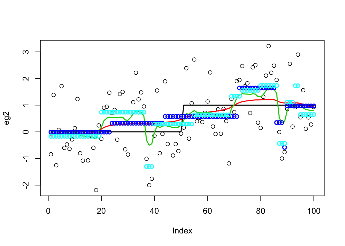

plot(colMeans(eg2.bcp.long$mcmc.means),col=4)
lines(eg2.bcp$posterior.mean)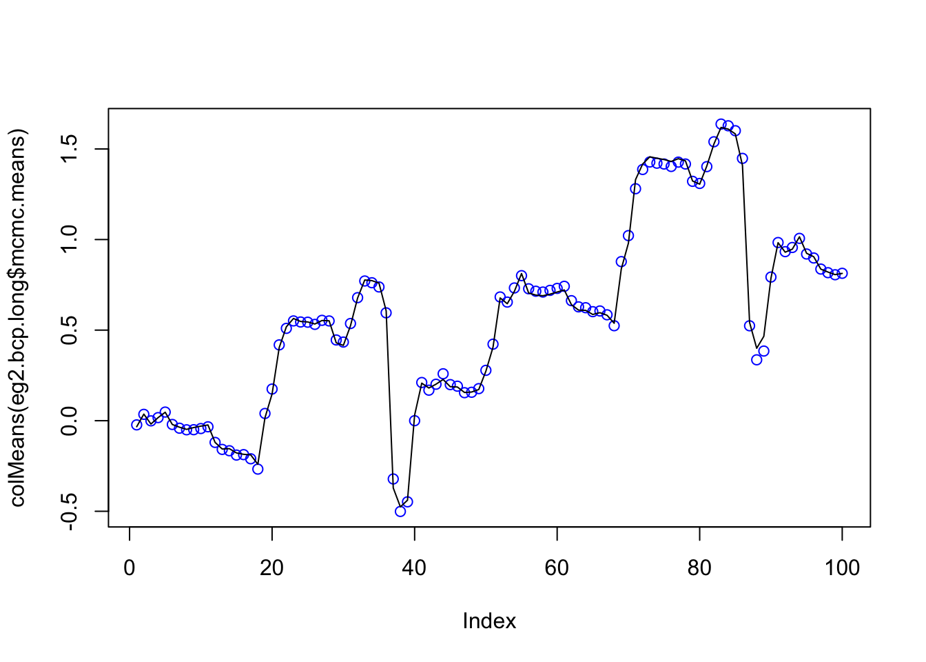

That is suprising that the long and short run agree so closely. But

eg2.bcp.short <- bcp(eg2,mcmc=100,return.mcmc=TRUE)
plot(eg2.bcp.short$posterior.mean,eg2.bcp$posterior.mean)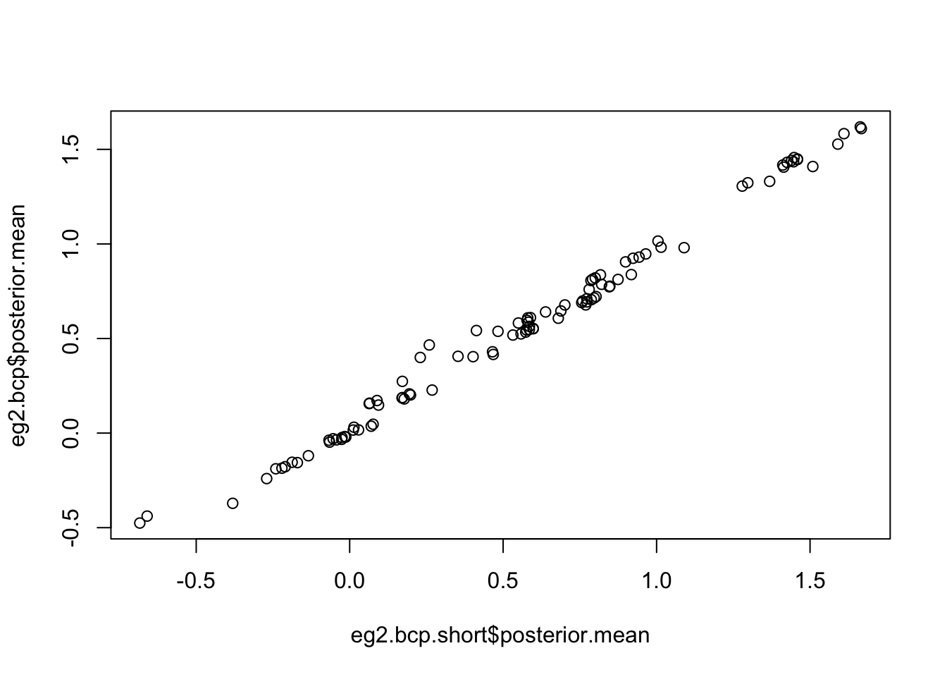

DNA segmentation example from bcp package

This example comes from demo(coriell) in the bcp package.

data(coriell)
chrom11 <- as.vector(na.omit(coriell$Coriell.05296[coriell$Chromosome==11]))
chrom11.bcp <- bcp(chrom11)
plot(chrom11.bcp, main="Coriell chromosome 11 (bcp)")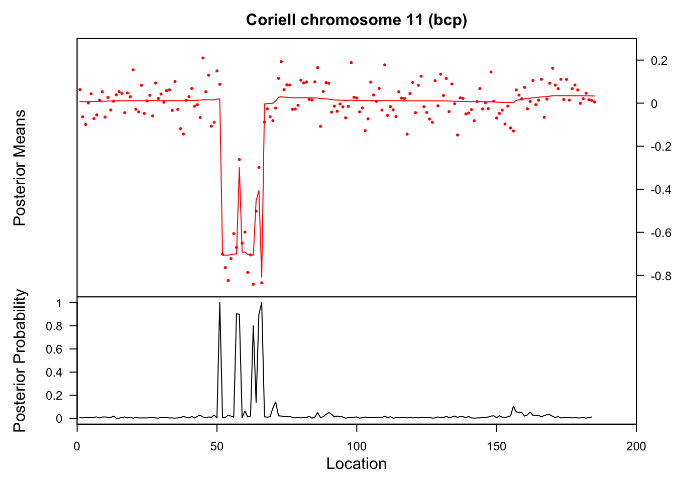

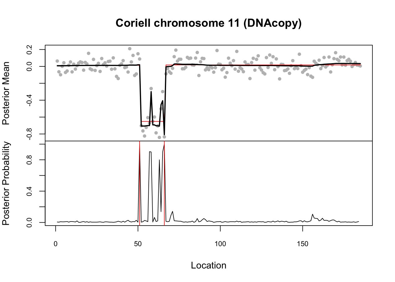
Here it compares results with DNAcopy package (also part of the demo)

  library("DNAcopy")
   n <- length(chrom11)
   cbs <- segment(CNA(chrom11, rep(1, n), 1:n), verbose = 0)
   cbs.ests <- rep(unlist(cbs$output[6]), unlist(cbs$output[5]))
   op <- par(mfrow=c(2,1),col.lab="black",col.main="black")
   op2 <- par(mar=c(0,4,4,2),xaxt="n", cex.axis=0.75)
   plot(1:n, chrom11.bcp$data[,2], col="grey", pch=20, xlab="Location",
        ylab="Posterior Mean",
        main="Coriell chromosome 11 (DNAcopy)")
   lines(cbs.ests, col="red")
   lines(chrom11.bcp$posterior.mean, lwd=2)
   par(op2)
   op3 <- par(mar=c(5,4,0,2), xaxt="s", cex.axis=0.75)
   plot(1:n, chrom11.bcp$posterior.prob, type="l", ylim=c(0,1),
        xlab="Location", ylab="Posterior Probability", main="")
   for (i in 1:(dim(cbs$output)[1]-1)) {
     abline(v=cbs$output$loc.end[i], col="red")
   }

   par(op3)
   par(op)

Try susie. Note that this example illustrates a case where a variable (here 66) occurs in multiple CSs… something we don’t yet fully understand the implications of I think.

  chrom11.s = susie_cp(chrom11)
  plot(1:n, chrom11, col="grey", pch=20, xlab="Location",
        ylab="Posterior Mean",
        main="Coriell chromosome 11 (DNAcopy)")
  lines(predict(chrom11.s),col=2,lwd=2)
  chrom11.s$sets

$cs
$cs$L2
[1] 51

$cs$L3
[1] 66

$cs$L4
[1] 63 64 66

$cs$L1
[1] 66 67 68 69 70 71


$purity
   min.abs.corr mean.abs.corr median.abs.corr
L2    1.0000000     1.0000000       1.0000000
L3    1.0000000     1.0000000       1.0000000
L4    0.9649213     0.9843474       0.9880822
L1    0.9436735     0.9778424       0.9772150

$cs_index
[1] 2 3 4 1

$coverage
[1] 0.95

  abline(v=66)
  abline(v=51)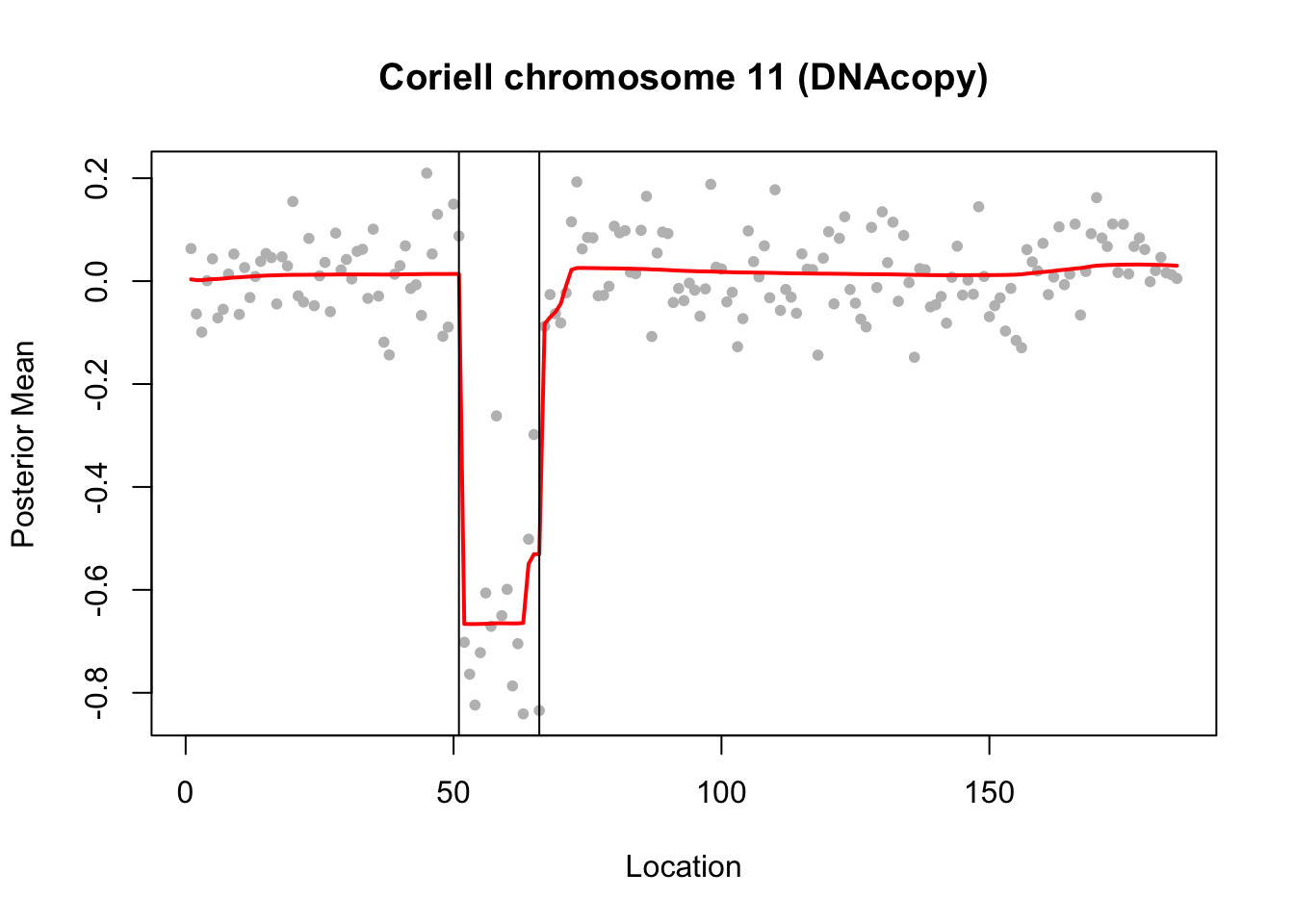

An example from the DNAcopy segment function:

set.seed(51)
true_mean = rep(c(-0.2,0.1,1,-0.5,0.2,-0.5,0.1,-0.2),c(137,87,17,49,29,52,87,42))
genomdat <- rnorm(500, sd=0.2) + true_mean

plot(genomdat)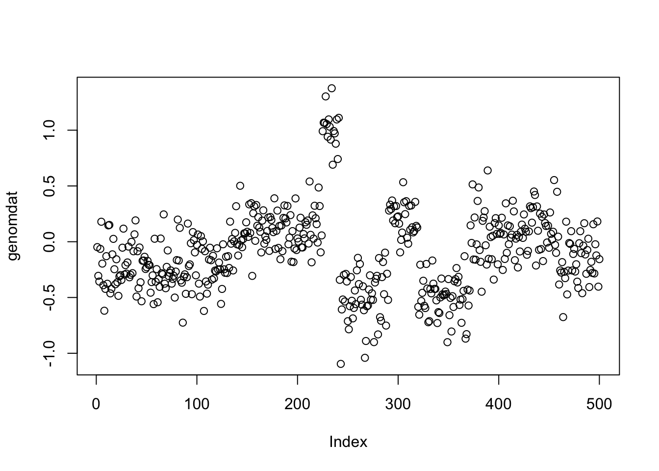

chrom <- rep(1:2,c(290,210))
maploc <- c(1:290,1:210)

genomdat.seg <- segment(CNA(genomdat, chrom, maploc))

Analyzing: Sample.1 

plot(genomdat.seg)
genomdat.s = susie_cp(genomdat)


plot_cs(genomdat.s)    
lines(true_mean,col=1,type="s")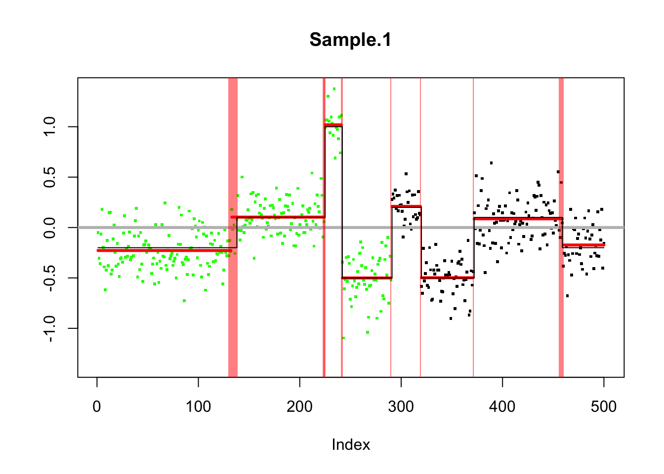

plot(genomdat.s$pip)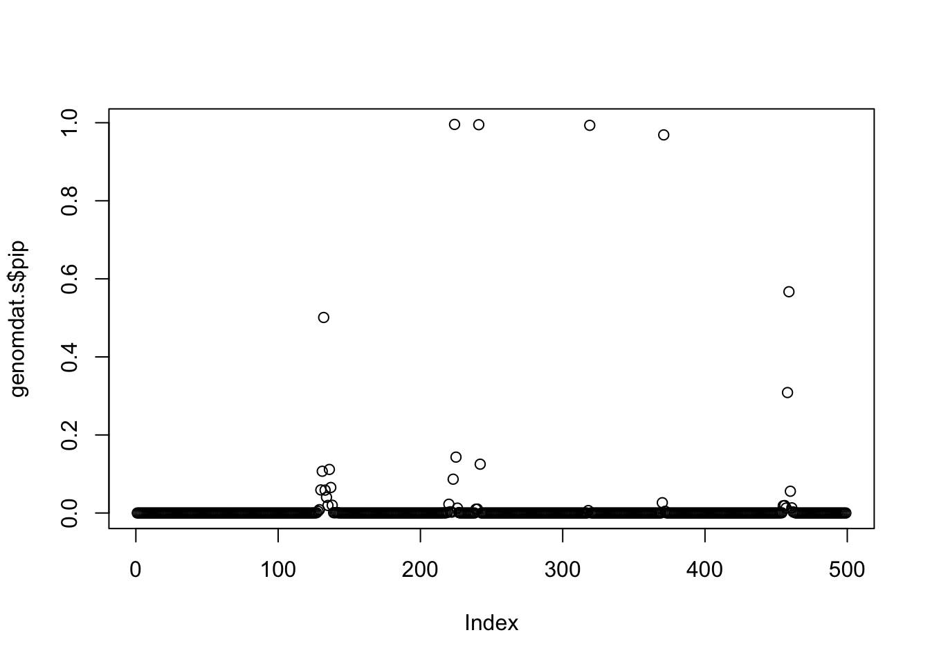

genomdat.bcp = bcp(genomdat)
plot(genomdat.bcp)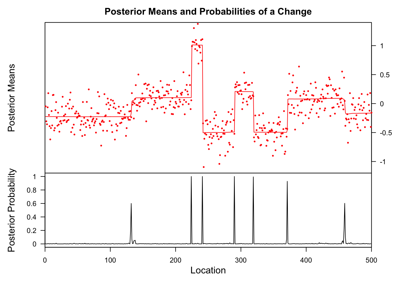

plot(genomdat.bcp$posterior.mean,predict(genomdat.s))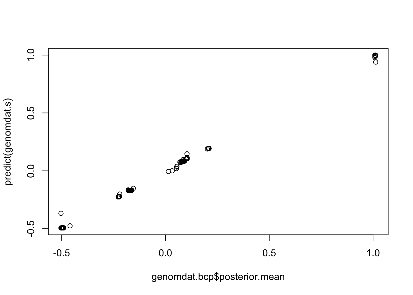

This example from DNAcopy too. (commented out for now as takes too long.)

# data(coriell)
# 
# #Combine into one CNA object to prepare for analysis on Chromosomes 1-23
# 
# CNA.object <-CNA(cbind(coriell$Coriell.05296,coriell$Coriell.13330),coriell$Chromosome,coriell$Position,data.type="logratio",sampleid=c("c05296","c13330"))
# 
# s = susie_cp(CNA.object$c13330[!is.na(CNA.object$c13330)])
# plot(CNA.object$c13330[!is.na(CNA.object$c13330)])
# plot_cs(s)

Session information

sessionInfo()

R version 3.5.1 (2018-07-02)
Platform: x86_64-apple-darwin15.6.0 (64-bit)
Running under: OS X El Capitan 10.11.6

Matrix products: default
BLAS: /Library/Frameworks/R.framework/Versions/3.5/Resources/lib/libRblas.0.dylib
LAPACK: /Library/Frameworks/R.framework/Versions/3.5/Resources/lib/libRlapack.dylib

locale:
[1] en_US.UTF-8/en_US.UTF-8/en_US.UTF-8/C/en_US.UTF-8/en_US.UTF-8

attached base packages:
[1] grid      stats     graphics  grDevices utils     datasets  methods  
[8] base     

other attached packages:
[1] DNAcopy_1.55.0    genlasso_1.4      igraph_1.2.2      Matrix_1.2-14    
[5] bcp_4.0.3         susieR_0.5.0.0347 changepoint_2.2.2 zoo_1.8-4        

loaded via a namespace (and not attached):
 [1] Rcpp_0.12.19       knitr_1.20         whisker_0.3-2     
 [4] magrittr_1.5       workflowr_1.1.1    lattice_0.20-35   
 [7] stringr_1.3.1      tools_3.5.1        R.oo_1.22.0       
[10] git2r_0.23.0       htmltools_0.3.6    matrixStats_0.54.0
[13] yaml_2.2.0         rprojroot_1.3-2    digest_0.6.18     
[16] R.utils_2.7.0      evaluate_0.12      rmarkdown_1.10    
[19] stringi_1.2.4      compiler_3.5.1     backports_1.1.2   
[22] R.methodsS3_1.7.1  pkgconfig_2.0.2