Differential expression analysis
Siming Zhao
December 2, 2018
Last updated: 2018-12-05
workflowr checks: (Click a bullet for more information)-
✖ R Markdown file: uncommitted changes
The R Markdown is untracked by Git. To know which version of the R Markdown file created these results, you’ll want to first commit it to the Git repo. If you’re still working on the analysis, you can ignore this warning. When you’re finished, you can runwflow_publishto commit the R Markdown file and build the HTML. -
✔ Environment: empty
Great job! The global environment was empty. Objects defined in the global environment can affect the analysis in your R Markdown file in unknown ways. For reproduciblity it’s best to always run the code in an empty environment.
-
✔ Seed:
set.seed(20181119)The command
set.seed(20181119)was run prior to running the code in the R Markdown file. Setting a seed ensures that any results that rely on randomness, e.g. subsampling or permutations, are reproducible. -
✔ Session information: recorded
Great job! Recording the operating system, R version, and package versions is critical for reproducibility.
-
Great! You are using Git for version control. Tracking code development and connecting the code version to the results is critical for reproducibility. The version displayed above was the version of the Git repository at the time these results were generated.✔ Repository version: 275d5d8
Note that you need to be careful to ensure that all relevant files for the analysis have been committed to Git prior to generating the results (you can usewflow_publishorwflow_git_commit). workflowr only checks the R Markdown file, but you know if there are other scripts or data files that it depends on. Below is the status of the Git repository when the results were generated:
Note that any generated files, e.g. HTML, png, CSS, etc., are not included in this status report because it is ok for generated content to have uncommitted changes.Ignored files: Ignored: .Rhistory Ignored: .Rproj.user/ Ignored: analysis/Quality_metrics_cache/ Ignored: analysis/figure/ Untracked files: Untracked: analysis/DE_analysis.Rmd Untracked: code/qq-plot.R Untracked: code/summary_functions.R Untracked: docs/figure/DE_analysis.Rmd/ Unstaged changes: Modified: analysis/Quality_metrics.Rmd Modified: analysis/crop_workflow_Alan.Rmd Modified: analysis/index.Rmd Modified: data/DE_input.Rd
Load data
source("code/summary_functions.R")
load("data/DE_input.Rd")
glocus <- "VPS45"
dim(dm)[1]NULLgcount <- dm[1:(dim(dm)[1]-76), colnames(dm1dfagg)[dm1dfagg[glocus,] >0 & nlocus==1]]
# negative control cells defined as neg gRNA targeted cells
ncount <- dm[1:(dim(dm)[1]-76), colnames(dm1dfagg)[dm1dfagg["neg",] >0 & nlocus==1]]
coldata <- data.frame(row.names = c(colnames(gcount),colnames(ncount)),
condition=c(rep('G',dim(gcount)[2]),rep('N',dim(ncount)[2])))DEseq2
standard DESeq2
library(DESeq2)
dds = DESeqDataSetFromMatrix(countData = cbind(gcount,ncount),
                             colData = coldata,
                             design = ~condition)

dds = estimateSizeFactors(dds)
ddsWARD = DESeq(dds)
resWARD = results(ddsWARD)
summ_pvalues(resWARD$pvalue[!is.na(resWARD$pvalue)])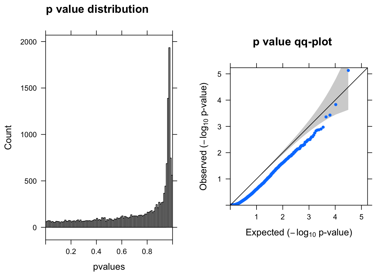
resSigWARD <- subset(resWARD, padj < 0.1)There are 0 genes passed FDR <0.1 cutoff.
DESeq2 with LRT test
Following recommendation for single cell from here.
ddsLRT = DESeq(dds, test="LRT", reduced = ~1,  sfType="poscounts", useT=TRUE, minmu=1e-6,minReplicatesForReplace=Inf)
resLRT = results(ddsLRT)
summ_pvalues(resLRT$pvalue[!is.na(resLRT$pvalue)])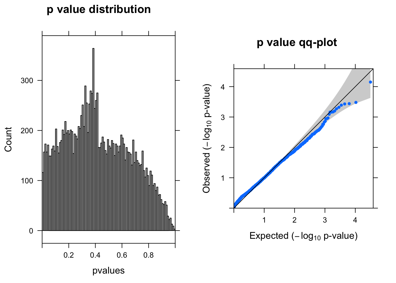
resSigLRT <- subset(resLRT, padj < 0.1)There are 0 genes passed FDR <0.1 cutoff.
edgeR
quasi-likelihood F-tests
library(edgeR)
y <- DGEList(counts= cbind(gcount,ncount),group=coldata$condition)
y <- calcNormFactors(y)
group=coldata$condition
design <- model.matrix(~group)
y <- estimateDisp(y,design)
fitqlf <- glmQLFit(y,design)
qlf <- glmQLFTest(fitqlf,coef=2)
summ_pvalues(qlf$table$PValue)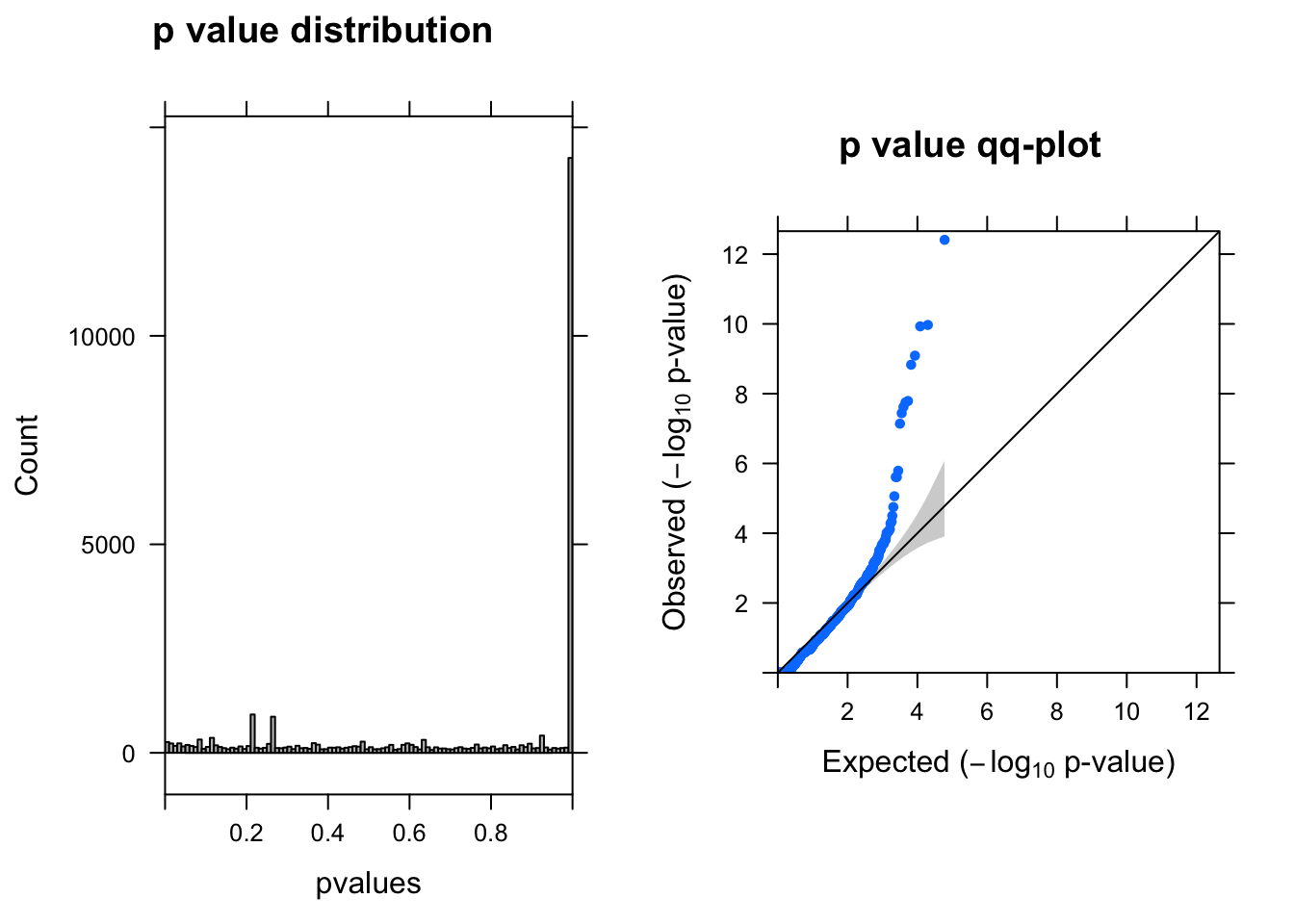
topTags(qlf)Coefficient: groupN
logFC logCPM F PValue FDR
ENSG00000176956.12 -2.776350 6.601479 58.72481 3.918884e-13 1.169630e-08
ENSG00000100097.11 -2.299929 6.624158 45.44607 1.064435e-10 1.171374e-06
ENSG00000130203.9 -1.831334 6.391155 45.21290 1.177418e-10 1.171374e-06
ENSG00000100300.17 -1.607537 6.410639 40.80264 8.073546e-10 6.024077e-06
ENSG00000138136.6 -1.976572 6.423656 39.44806 1.468212e-09 8.764051e-06
ENSG00000089116.3 -1.542926 6.320288 36.99506 1.605330e-08 7.578892e-05
ENSG00000175899.14 -1.584250 6.857262 33.87858 1.777533e-08 7.578892e-05
ENSG00000162992.3 -1.608906 6.373881 34.49478 2.385458e-08 8.899547e-05
ENSG00000198417.6 -1.600763 6.403261 32.30436 3.635396e-08 1.205578e-04
ENSG00000104327.7 -1.374926 6.326720 49.50835 7.206623e-08 2.150889e-04likelihood ratio tests
fitlrt <- glmFit(y,design)
lrt <- glmLRT(fitlrt,coef=2)
topTags(lrt)
Coefficient: groupN
logFC logCPM LR PValue FDR
ENSG00000175899.14 -1.4640348 6.857262 19.83212 8.454987e-06 0.1170441
ENSG00000176956.12 -2.6064930 6.601479 19.25383 1.144407e-05 0.1170441
ENSG00000100097.11 -2.2150044 6.624158 19.20106 1.176480e-05 0.1170441
ENSG00000100300.17 -1.4959097 6.410639 14.35365 1.514859e-04 0.9651347
ENSG00000119906.11 1.0518706 6.444915 13.90103 1.926926e-04 0.9651347
ENSG00000185900.9 -0.7876253 6.269218 13.68055 2.166870e-04 0.9651347
ENSG00000219626.8 -0.9907215 6.458688 13.59855 2.263601e-04 0.9651347
ENSG00000078061.12 -0.8304381 6.581079 12.89330 3.297606e-04 1.0000000
ENSG00000234912.11 1.0422011 6.412729 12.49191 4.087177e-04 1.0000000
ENSG00000175806.14 -0.7904605 6.612756 12.19362 4.795325e-04 1.0000000summ_pvalues(lrt$table$PValue)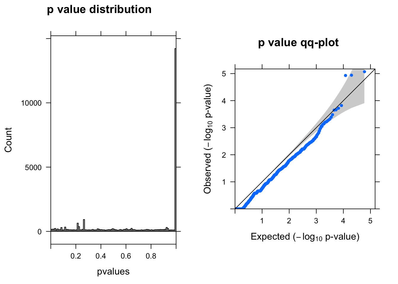
quasi-likelihood F-tests with prefiltering
Filter genes with 0 coverage in all cells.
mycount <- cbind(gcount,ncount)
totalcount <- apply(mycount,1,sum)
y <- DGEList(counts= mycount[totalcount>0,],group=coldata$condition)
y <- calcNormFactors(y)
group=coldata$condition
design <- model.matrix(~group)
y <- estimateDisp(y,design)
fitqlf <- glmQLFit(y,design)
qlf <- glmQLFTest(fitqlf,coef=2)
topTags(qlf)
Coefficient: groupN
logFC logCPM F PValue FDR
ENSG00000176956.12 -2.776350 6.601479 58.72481 3.918884e-13 6.170676e-09
ENSG00000100097.11 -2.299929 6.624158 45.44607 1.064435e-10 6.179874e-07
ENSG00000130203.9 -1.831334 6.391155 45.21290 1.177418e-10 6.179874e-07
ENSG00000100300.17 -1.607537 6.410639 40.80264 8.073546e-10 3.178152e-06
ENSG00000138136.6 -1.976572 6.423656 39.44806 1.468212e-09 4.623693e-06
ENSG00000089116.3 -1.542926 6.320288 36.99506 1.605330e-08 3.998433e-05
ENSG00000175899.14 -1.584250 6.857262 33.87858 1.777533e-08 3.998433e-05
ENSG00000162992.3 -1.608906 6.373881 34.49478 2.385458e-08 4.695177e-05
ENSG00000198417.6 -1.600763 6.403261 32.30436 3.635396e-08 6.360327e-05
ENSG00000104327.7 -1.374926 6.326720 49.50835 7.206623e-08 1.134755e-04summ_pvalues(qlf$table$PValue)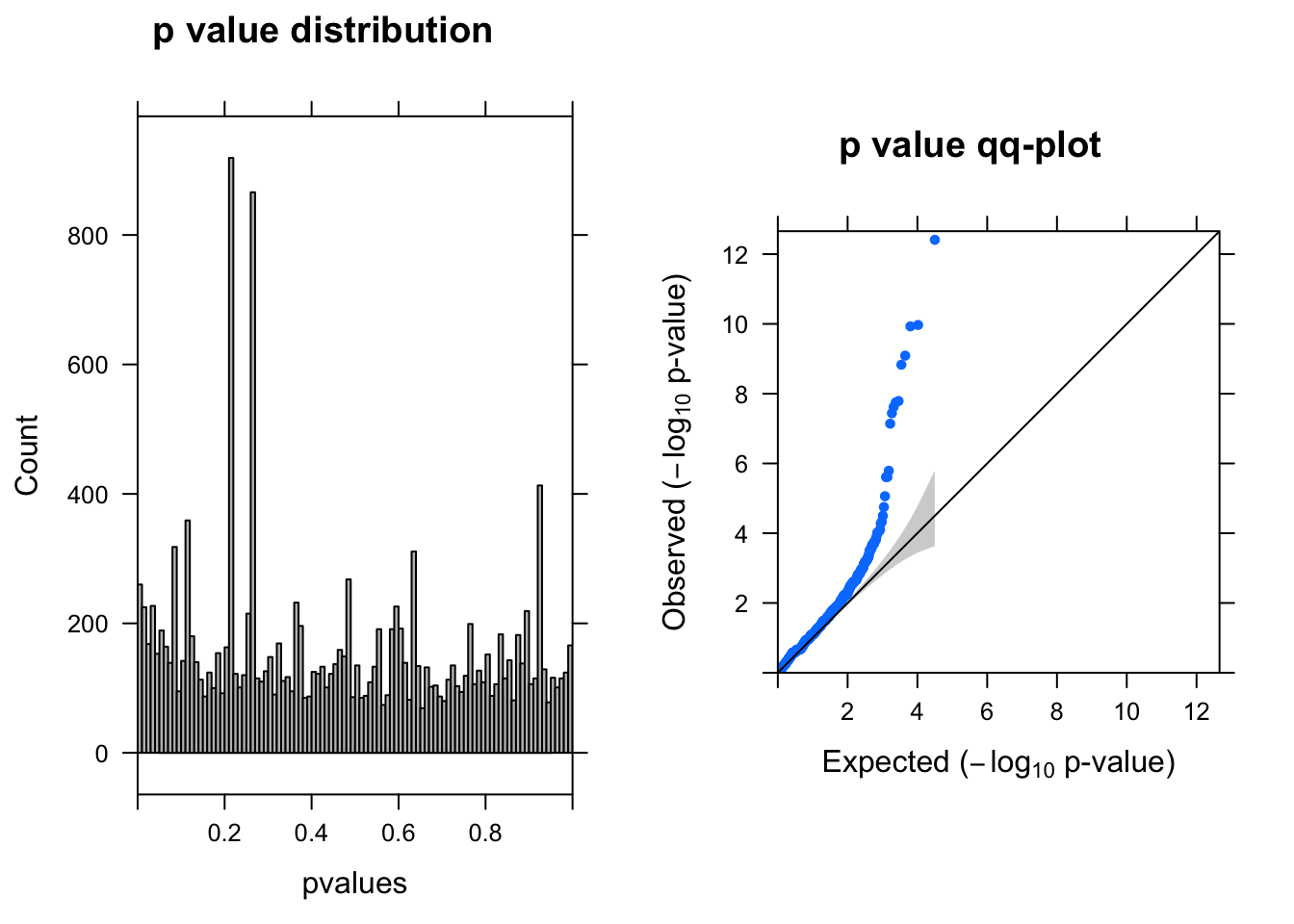
likelihood ratio tests with prefiltering
Filter genes with 0 coverage in all cells.
fitlrt <- glmFit(y,design)
lrt <- glmLRT(fitlrt,coef=2)
topTags(lrt)
Coefficient: groupN
logFC logCPM LR PValue FDR
ENSG00000175899.14 -1.4640348 6.857262 19.83212 8.454987e-06 0.06174953
ENSG00000176956.12 -2.6064930 6.601479 19.25383 1.144407e-05 0.06174953
ENSG00000100097.11 -2.2150044 6.624158 19.20106 1.176480e-05 0.06174953
ENSG00000100300.17 -1.4959097 6.410639 14.35365 1.514859e-04 0.50918085
ENSG00000119906.11 1.0518706 6.444915 13.90103 1.926926e-04 0.50918085
ENSG00000185900.9 -0.7876253 6.269218 13.68055 2.166870e-04 0.50918085
ENSG00000219626.8 -0.9907215 6.458688 13.59855 2.263601e-04 0.50918085
ENSG00000078061.12 -0.8304381 6.581079 12.89330 3.297606e-04 0.64905134
ENSG00000234912.11 1.0422011 6.412729 12.49191 4.087177e-04 0.66841632
ENSG00000175806.14 -0.7904605 6.612756 12.19362 4.795325e-04 0.66841632summ_pvalues(lrt$table$PValue)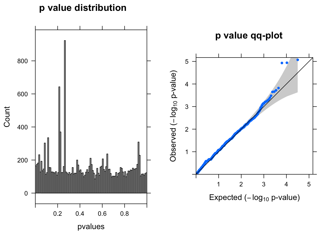
Parameters used
- We used data processed after QC step here.
- EdgeR: Prefiltering of lowly expressed genes: genes with 0 coverage in all cells. DEseq2 suggests that this pre-filtering step is only useful to increase speed, not for multiple testing purposes, so no filtering.
- targeted locus, choose VPS45.
Session information
sessionInfo()R version 3.5.1 (2018-07-02)
Platform: x86_64-apple-darwin14.5.0 (64-bit)
Running under: OS X El Capitan 10.11.6
Matrix products: default
BLAS: /System/Library/Frameworks/Accelerate.framework/Versions/A/Frameworks/vecLib.framework/Versions/A/libBLAS.dylib
LAPACK: /System/Library/Frameworks/Accelerate.framework/Versions/A/Frameworks/vecLib.framework/Versions/A/libLAPACK.dylib
locale:
[1] en_US.UTF-8/en_US.UTF-8/en_US.UTF-8/C/en_US.UTF-8/en_US.UTF-8
attached base packages:
[1] grid parallel stats4 stats graphics grDevices utils
[8] datasets methods base
other attached packages:
[1] edgeR_3.22.5 limma_3.36.5
[3] gridExtra_2.3 lattice_0.20-35
[5] DESeq2_1.20.0 SummarizedExperiment_1.10.1
[7] DelayedArray_0.6.6 BiocParallel_1.14.2
[9] matrixStats_0.54.0 Biobase_2.40.0
[11] GenomicRanges_1.32.7 GenomeInfoDb_1.16.0
[13] IRanges_2.14.12 S4Vectors_0.18.3
[15] BiocGenerics_0.26.0 Matrix_1.2-14
loaded via a namespace (and not attached):
[1] bit64_0.9-7 splines_3.5.1 R.utils_2.7.0
[4] Formula_1.2-3 assertthat_0.2.0 latticeExtra_0.6-28
[7] blob_1.1.1 GenomeInfoDbData_1.1.0 yaml_2.2.0
[10] RSQLite_2.1.1 pillar_1.3.0 backports_1.1.2
[13] glue_1.3.0 digest_0.6.18 RColorBrewer_1.1-2
[16] XVector_0.20.0 checkmate_1.8.5 colorspace_1.3-2
[19] htmltools_0.3.6 R.oo_1.22.0 plyr_1.8.4
[22] XML_3.98-1.16 pkgconfig_2.0.2 genefilter_1.62.0
[25] zlibbioc_1.26.0 purrr_0.2.5 xtable_1.8-3
[28] scales_1.0.0 whisker_0.3-2 git2r_0.23.0
[31] tibble_1.4.2 htmlTable_1.12 annotate_1.58.0
[34] ggplot2_3.1.0 nnet_7.3-12 lazyeval_0.2.1
[37] survival_2.42-6 magrittr_1.5 crayon_1.3.4
[40] memoise_1.1.0 evaluate_0.12 R.methodsS3_1.7.1
[43] foreign_0.8-71 tools_3.5.1 data.table_1.11.6
[46] stringr_1.3.1 locfit_1.5-9.1 munsell_0.5.0
[49] cluster_2.0.7-1 AnnotationDbi_1.42.1 bindrcpp_0.2.2
[52] compiler_3.5.1 rlang_0.3.0.1 RCurl_1.95-4.11
[55] rstudioapi_0.8 htmlwidgets_1.2 bitops_1.0-6
[58] base64enc_0.1-3 rmarkdown_1.10 gtable_0.2.0
[61] DBI_1.0.0 R6_2.3.0 knitr_1.20
[64] dplyr_0.7.6 bit_1.1-12 bindr_0.1.1
[67] Hmisc_4.1-1 workflowr_1.1.1 rprojroot_1.3-2
[70] stringi_1.2.4 Rcpp_1.0.0 geneplotter_1.58.0
[73] rpart_4.1-13 acepack_1.4.1 tidyselect_0.2.4 This reproducible R Markdown analysis was created with workflowr 1.1.1