Compare CENTIPEDE predictions for HIF1A
Kaixuan Luo
6/18/2018
Last updated: 2018-06-20
workflowr checks: (Click a bullet for more information)-
✔ R Markdown file: up-to-date
Great! Since the R Markdown file has been committed to the Git repository, you know the exact version of the code that produced these results.
-
✔ Environment: empty
Great job! The global environment was empty. Objects defined in the global environment can affect the analysis in your R Markdown file in unknown ways. For reproduciblity it’s best to always run the code in an empty environment.
-
✔ Seed:
set.seed(20180613)The command
set.seed(20180613)was run prior to running the code in the R Markdown file. Setting a seed ensures that any results that rely on randomness, e.g. subsampling or permutations, are reproducible. -
✔ Session information: recorded
Great job! Recording the operating system, R version, and package versions is critical for reproducibility.
-
Great! You are using Git for version control. Tracking code development and connecting the code version to the results is critical for reproducibility. The version displayed above was the version of the Git repository at the time these results were generated.✔ Repository version: 84a6174
Note that you need to be careful to ensure that all relevant files for the analysis have been committed to Git prior to generating the results (you can usewflow_publishorwflow_git_commit). workflowr only checks the R Markdown file, but you know if there are other scripts or data files that it depends on. Below is the status of the Git repository when the results were generated:
Note that any generated files, e.g. HTML, png, CSS, etc., are not included in this status report because it is ok for generated content to have uncommitted changes.Ignored files: Ignored: .DS_Store Ignored: .Rhistory Ignored: .Rproj.user/ Untracked files: Untracked: analysis/ATACseq_footprinting_pipeline.Rmd Untracked: analysis/compare_centipede_predictions_CTCF.Rmd Untracked: code_RCC/ Untracked: docs/figure/ Untracked: workflow_setup.R
Expand here to see past versions:
| File | Version | Author | Date | Message |
|---|---|---|---|---|
| Rmd | 84a6174 | kevinlkx | 2018-06-20 | compare centipede predictions for HIF1A |
library(ggplot2)
library(grid)
library(gridExtra)
library(limma)
library(edgeR)
select TF
tf_name <- "HIF1A"
pwm_name <- "HIF1A::ARNT_MA0259.1_1e-4"

thresh_PostPr_bound <- 0.99
cat(pwm_name, "\n")
HIF1A::ARNT_MA0259.1_1e-4 load CENTIPEDE predictions
dir_predictions <- paste0("~/Dropbox/research//ATAC-seq/for_Olivia_Gray/results/centipede_predictions/", pwm_name)

## condition: N
bam_namelist_N <- c("N1_nomito_rdup.bam", "N2_nomito_rdup.bam", "N3_nomito_rdup.bam")

site_predictions_N.l <- vector("list", 3)
names(site_predictions_N.l) <- bam_namelist_N

for(i in 1:length(bam_namelist_N)){
  bam_basename <- tools::file_path_sans_ext(basename(bam_namelist_N[[i]]))
  site_predictions_N.l[[i]] <- read.table(paste0(dir_predictions, "/", pwm_name, "_", bam_basename, "_predictions.txt.gz"), header = T, stringsAsFactors = F)
}

CentPostPr_N.df <- data.frame(N1 = site_predictions_N.l[[1]]$CentPostPr,
                              N2 = site_predictions_N.l[[2]]$CentPostPr,
                              N3 = site_predictions_N.l[[3]]$CentPostPr)

CentLogRatios_N.df <- data.frame(N1 = site_predictions_N.l[[1]]$CentLogRatios,
                                 N2 = site_predictions_N.l[[2]]$CentLogRatios,
                                 N3 = site_predictions_N.l[[3]]$CentLogRatios)


## condition: H
bam_namelist_H <- c("H1_nomito_rdup.bam", "H2_nomito_rdup.bam", "H3_nomito_rdup.bam")

site_predictions_H.l <- vector("list", 3)
names(site_predictions_H.l) <- bam_namelist_H

for(i in 1:length(bam_namelist_H)){
  bam_basename <- tools::file_path_sans_ext(basename(bam_namelist_H[[i]]))
  site_predictions_H.l[[i]] <- read.table(paste0(dir_predictions, "/", pwm_name, "_", bam_basename, "_predictions.txt.gz"), header = T, stringsAsFactors = F)
}

name_sites <- site_predictions_H.l[[1]]$name

CentPostPr_H.df <- data.frame(H1 = site_predictions_H.l[[1]]$CentPostPr,
                              H2 = site_predictions_H.l[[2]]$CentPostPr,
                              H3 = site_predictions_H.l[[3]]$CentPostPr)

CentLogRatios_H.df <- data.frame(H1 = site_predictions_H.l[[1]]$CentLogRatios,
                                 H2 = site_predictions_H.l[[2]]$CentLogRatios,
                                 H3 = site_predictions_H.l[[3]]$CentLogRatios)

CentPostPr.df <- cbind(CentPostPr_N.df, CentPostPr_H.df)
CentLogRatios.df <- cbind(CentLogRatios_N.df, CentLogRatios_H.df)
binarize to bound and unbound
cat("Number of bound sites: \n")Number of bound sites: colSums(CentPostPr.df > thresh_PostPr_bound) N1 N2 N3 H1 H2 H3
4139 3834 3539 2334 2213 2788 idx_bound <- which(rowSums(CentPostPr.df > thresh_PostPr_bound) >= 2)
cat(length(idx_bound), "sites are bound in at least two samples \n")3882 sites are bound in at least two samples cat(length(idx_bound), "(",round(length(idx_bound)/nrow(CentPostPr.df) *100, 2), "% ) sites are bound in at least two samples \n")3882 ( 6.85 % ) sites are bound in at least two samples Plot average binding and average logRatios
all sites
par(pty="s")
plot(rowMeans(CentPostPr_N.df), rowMeans(CentPostPr_H.df),
     xlab = "N average P(Bound)", ylab = "H average P(Bound)", main = tf_name,
     pch = ".", col = rgb(0,0,1,0.7))
abline(a=0,b=1)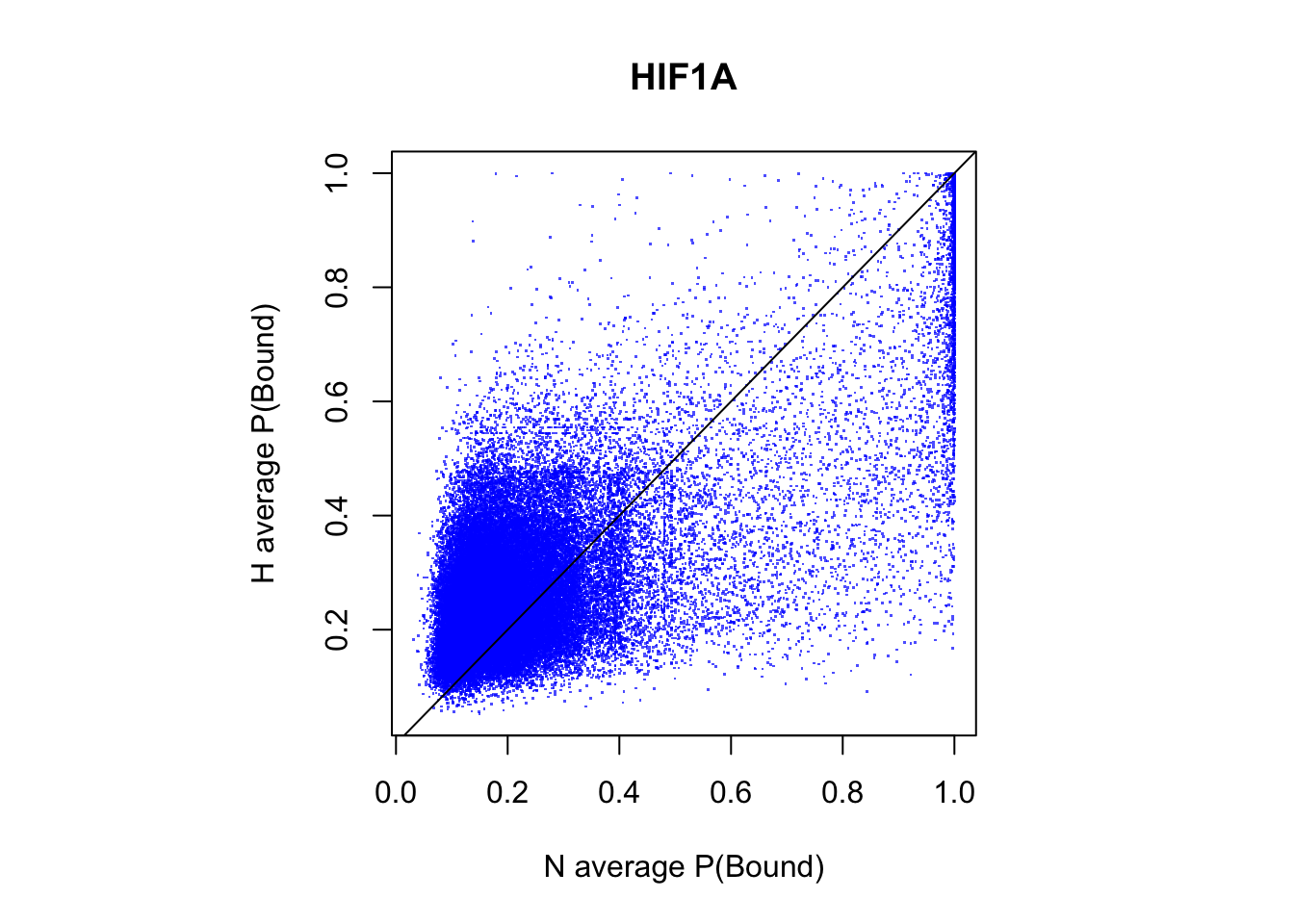
par(mfrow = c(1,2))
par(pty="s")
plot(rowMeans(CentLogRatios_N.df), rowMeans(CentLogRatios_H.df),
     xlab = "N average logRatios", ylab = "H average logRatios", main = tf_name,
     pch = ".", col = rgb(0,0,1,0.7))
abline(a=0,b=1,col = "darkgray")

plot(x = (rowMeans(CentLogRatios_H.df)+rowMeans(CentLogRatios_N.df))/2,
     y = rowMeans(CentLogRatios_H.df) - rowMeans(CentLogRatios_N.df),
     xlab = "average logRatios", ylab = "Difference in logRatios (H - N)", main = tf_name,
     pch = ".", col = rgb(0,0,1,0.7))
abline(v=0, h=0, col = "darkgray")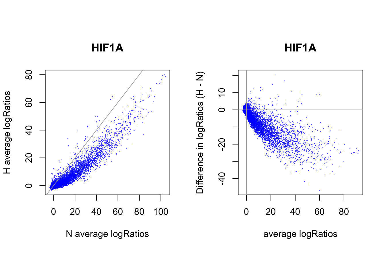
bound sites
par(pty="s")
plot(rowMeans(CentPostPr_N.df[idx_bound,]), rowMeans(CentPostPr_H.df[idx_bound,]),
     xlab = "N average P(Bound)", ylab = "H average P(Bound)", main = paste(tf_name, "bound sites"),
     pch = ".", col = rgb(0,0,1,0.7))
abline(a=0,b=1)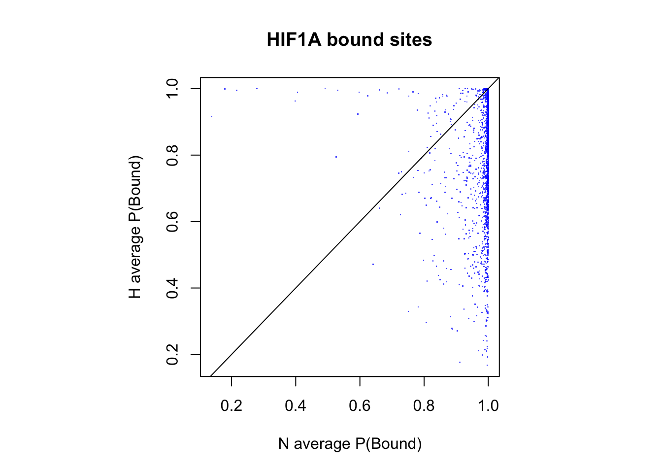
par(mfrow = c(1,2))
par(pty="s")
plot(rowMeans(CentLogRatios_N.df[idx_bound,]), rowMeans(CentLogRatios_H.df[idx_bound,]),
     xlab = "N average logRatios", ylab = "H average logRatios", main = tf_name,
     pch = ".", col = rgb(0,0,1,0.7))
abline(a=0,b=1,col = "darkgray")

plot(x = (rowMeans(CentLogRatios_H.df[idx_bound,])+rowMeans(CentLogRatios_N.df[idx_bound,]))/2,
     y = rowMeans(CentLogRatios_H.df[idx_bound,]) - rowMeans(CentLogRatios_N.df[idx_bound,]),
     xlab = "average logRatios", ylab = "Difference in logRatios (H - N)", main = tf_name,
     pch = ".", col = rgb(0,0,1,0.7))
abline(v=0, h=0, col = "darkgray")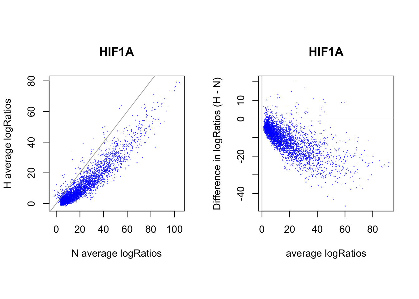
PCA
all sites
pca_logRatios <- prcomp(t(CentLogRatios.df))
percentage <- round(pca_logRatios$sdev / sum(pca_logRatios$sdev) * 100, 2)
percentage <- paste0( colnames(pca_logRatios$x), " (", paste( as.character(percentage), "%)") )

pca_logRatios.df <- as.data.frame(pca_logRatios$x)
pca_logRatios.df$group <- rep(c("N","H"), each = 3)
p <- ggplot(pca_logRatios.df, aes(x=PC1,y=PC2,color=group,label=row.names(pca_logRatios.df)))
p <- p + geom_point() + geom_text(size = 3, show.legend = F, vjust = 2, nudge_y = 0.5) +
  labs(title = tf_name, x = percentage[1], y = percentage[2])
p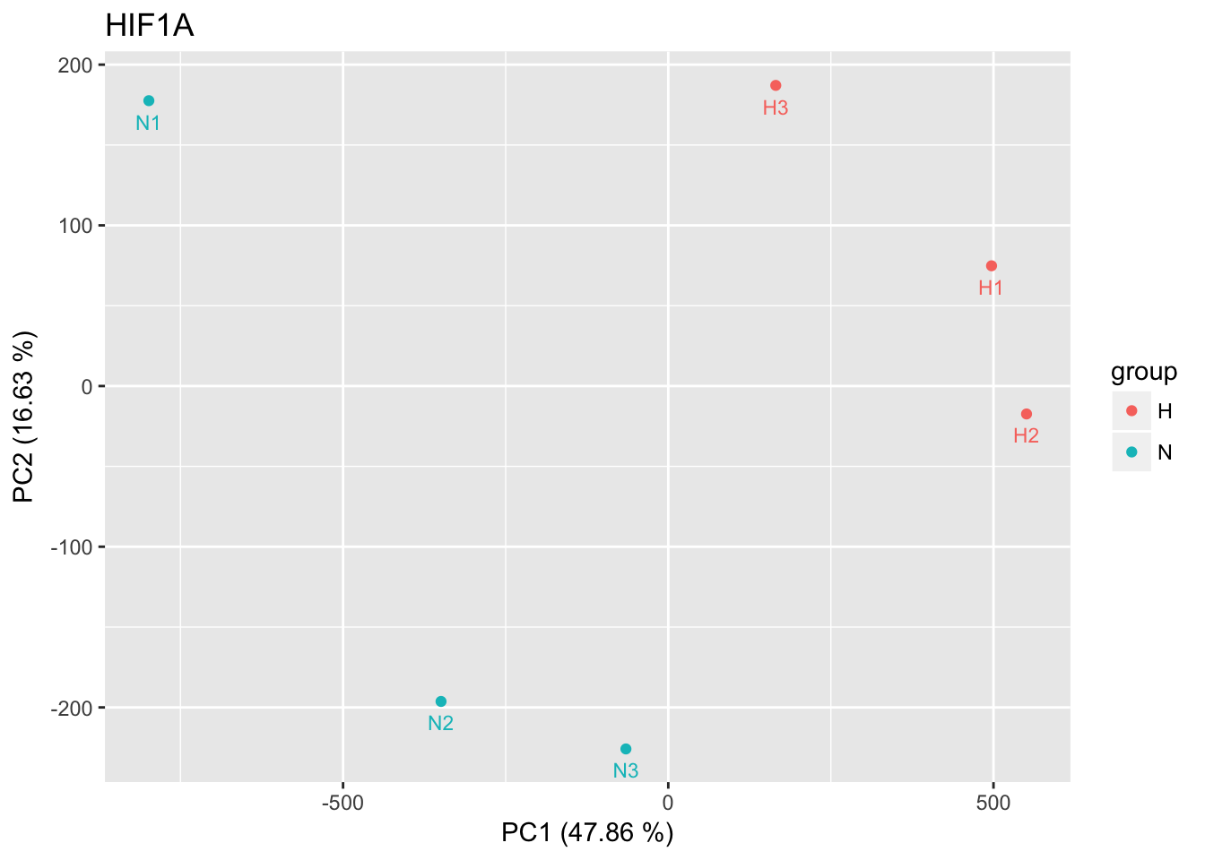
bound sites
pca_logRatios <- prcomp(t(CentLogRatios.df[idx_bound, ]))
percentage <- round(pca_logRatios$sdev / sum(pca_logRatios$sdev) * 100, 2)
percentage <- paste0( colnames(pca_logRatios$x), " (", paste( as.character(percentage), "%)") )

pca_logRatios.df <- as.data.frame(pca_logRatios$x)
pca_logRatios.df$group <- rep(c("N","H"), each = 3)
p <- ggplot(pca_logRatios.df, aes(x=PC1,y=PC2,color=group,label=row.names(pca_logRatios.df)))
p <- p + geom_point() + geom_text(size = 3, show.legend = F, vjust = 2, nudge_y = 0.5) +
  labs(title = tf_name, x = percentage[1], y = percentage[2])
p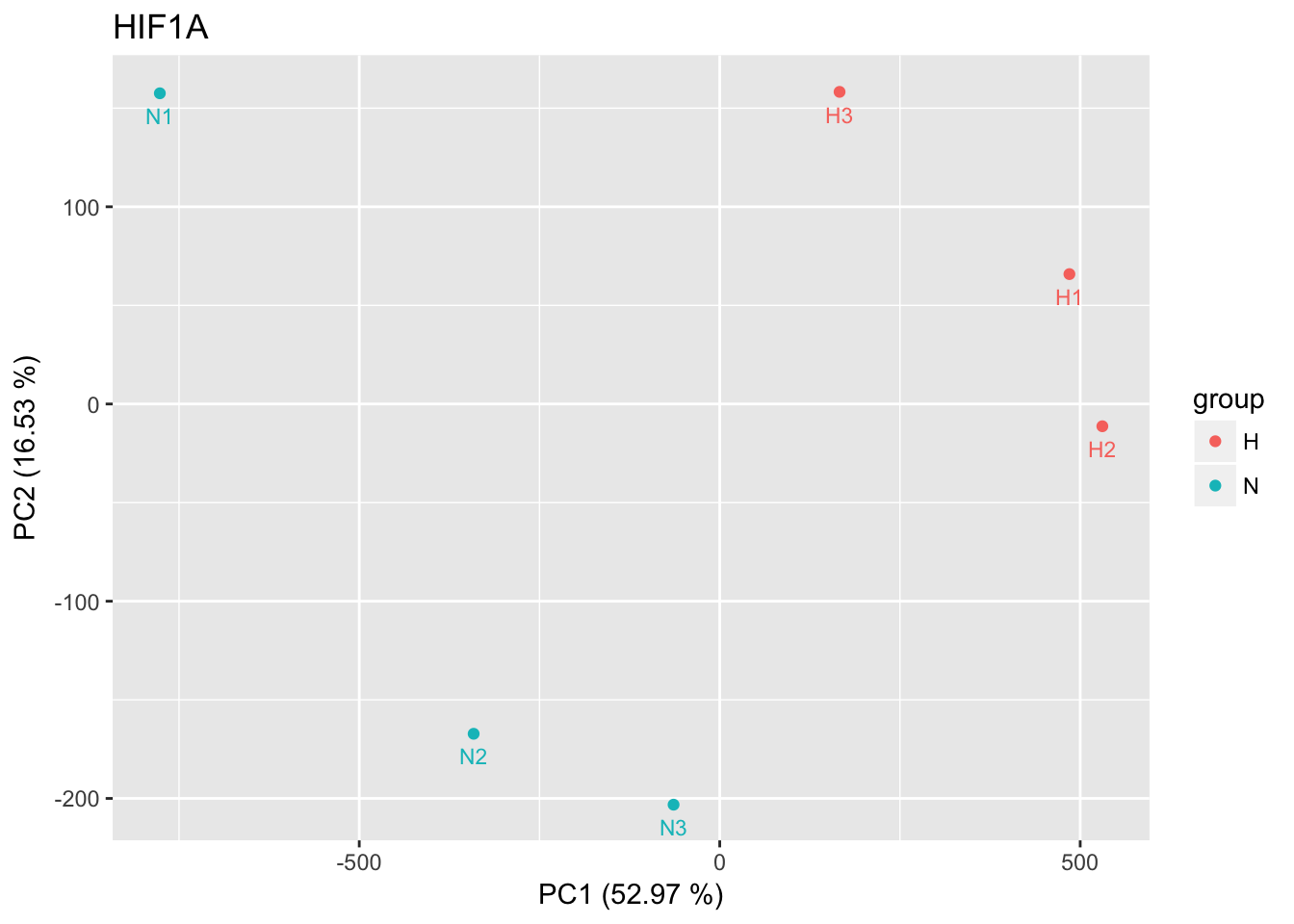
Differential logRatios for bound sites using limma
targets <- data.frame(bam = c(bam_namelist_N, bam_namelist_H),
                      label = colnames(CentLogRatios.df),
                      condition = rep(c("N", "H"), each = 3))

print(targets)
bam label condition
1 N1_nomito_rdup.bam N1 N
2 N2_nomito_rdup.bam N2 N
3 N3_nomito_rdup.bam N3 N
4 H1_nomito_rdup.bam H1 H
5 H2_nomito_rdup.bam H2 H
6 H3_nomito_rdup.bam H3 Hcondition <- factor(targets$condition, levels = c("N", "H"))
design <- model.matrix(~0+condition)
colnames(design) <- levels(condition)
print(design) N H
1 1 0
2 1 0
3 1 0
4 0 1
5 0 1
6 0 1
attr(,"assign")
[1] 1 1
attr(,"contrasts")
attr(,"contrasts")$condition
[1] "contr.treatment"CentLogRatios_Bound.df <- CentLogRatios.df[idx_bound, ]
fit <- lmFit(CentLogRatios_Bound.df, design)
contrasts <- makeContrasts(H-N, levels=design)
fit2 <- contrasts.fit(fit, contrasts)
fit2 <- eBayes(fit2, trend=TRUE)
num_diffbind <- summary(decideTests(fit2))
percent_diffbind <- round(num_diffbind / sum(num_diffbind) * 100, 2)
cat(percent_diffbind[1], "% down in H vs. N,", percent_diffbind[3], "% up in H vs. N \n")63.34 % down in H vs. N, 0.52 % up in H vs. N # volcanoplot(fit2, main="H vs. N", xlab = "Difference in logRatios (H - N)")
plot(x = fit2$coef, y = -log10(fit2$p.value),
xlab = "Difference in logRatios (H - N)", ylab = "-log10(P-value)", main= paste(tf_name, "H vs. N"),
pch = 16, cex = 0.35)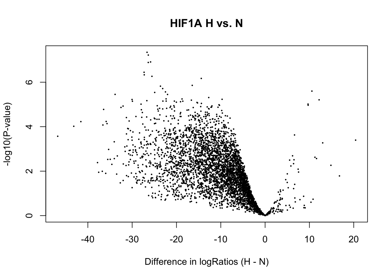
Session information
sessionInfo()R version 3.4.3 (2017-11-30)
Platform: x86_64-apple-darwin15.6.0 (64-bit)
Running under: macOS High Sierra 10.13.4
Matrix products: default
BLAS: /Library/Frameworks/R.framework/Versions/3.4/Resources/lib/libRblas.0.dylib
LAPACK: /Library/Frameworks/R.framework/Versions/3.4/Resources/lib/libRlapack.dylib
locale:
[1] en_US.UTF-8/en_US.UTF-8/en_US.UTF-8/C/en_US.UTF-8/en_US.UTF-8
attached base packages:
[1] grid stats graphics grDevices utils datasets methods
[8] base
other attached packages:
[1] edgeR_3.20.9 limma_3.34.9 gridExtra_2.3 ggplot2_2.2.1
loaded via a namespace (and not attached):
[1] Rcpp_0.12.16 knitr_1.20 whisker_0.3-2
[4] magrittr_1.5 workflowr_1.0.1 splines_3.4.3
[7] munsell_0.4.3 lattice_0.20-35 colorspace_1.3-2
[10] rlang_0.2.0 stringr_1.3.0 plyr_1.8.4
[13] tools_3.4.3 gtable_0.2.0 R.oo_1.22.0
[16] git2r_0.21.0 htmltools_0.3.6 yaml_2.1.18
[19] lazyeval_0.2.1 rprojroot_1.3-2 digest_0.6.15
[22] tibble_1.4.2 R.utils_2.6.0 evaluate_0.10.1
[25] rmarkdown_1.9 labeling_0.3 stringi_1.1.7
[28] pillar_1.2.2 compiler_3.4.3 scales_0.5.0
[31] backports_1.1.2 R.methodsS3_1.7.1 locfit_1.5-9.1 This reproducible R Markdown analysis was created with workflowr 1.0.1