CONFESS image classification: preliminary analysis
Last updated: 2017-10-12
Code version: 8e822f0
Background and goals
Here we use CONFESS to perform FUCCI and DAPI image analysis. CONFESS is built on EBImage and has been previously used to quantify cell cycle phase for 200+ HeLa cells. Their results are described in a bioRxiv paper (http://dx.doi.org/10.1101/088500).
In this document, I report results for four different FUCCI plates (18855_18511, 18870_18855, 18870_19101, 19101_19098). Additional results are reported for 18855_18511 comparing analysis on two sets of images differing in crop sizes.
Loading data and packages
Load RDS.
confess_18855_18511_crop1 <- readRDS(file = "../data/18855_18511_crop_09052017.rds")
confess_18855_18511_crop2 <- readRDS(file = "../data/18855_18511_crop_09072017.rds")
confess_18870_18855 <- readRDS(file = "../data/18870_18855_crop_09072017.rds")

confess_18870_19101 <- readRDS(file = "../data/18870_19101_crop_09122017.rds")
confess_19101_19098 <- readRDS(file = "../data/19101_19098_crop_09122017.rds")
Functions for exploratory data analysis.
# make three plots
# 1. log2 foreground versus log2 background intensity for Red channel
# 2. log2 foreground versus log2 background intensity for Green channel
# 3. signal-to-noise ratio of green versus red

eda <- function(data, plot_title) {
  with(data, {
    xlim_red <- ylim_red <- range(c(log2(back_Red), log2(fore_Red)))
    xlim_green <- ylim_green <- range(c(log2(back_Green), log2(fore_Green)))

    par(mfrow = c(2,2))
    plot(x = log2(back_Red), y = log2(fore_Red), pch = 16, cex = .7,
         xlim = xlim_red, ylim = ylim_red); abline(0, 1)
    plot(x = log2(back_Green), y = log2(fore_Green), pch = 16, cex = .7,
         xlim = xlim_green, ylim = ylim_green); abline(0, 1)
    StN.red <- log2(fore_Red) - min(log2(back_Red))
    StN.green <- log2(fore_Green) - min(log2(back_Green))
    StN.red.norm <- (StN.red-min(StN.red))/(max(StN.red)-min(StN.red))
    StN.green.norm <- (StN.green-min(StN.green))/(max(StN.green)-min(StN.green))
    plot(x = StN.green.norm, y = StN.red.norm,
         pch = 16, cex = .7); abline(v=.5, h = .5)
    title(main = plot_title, outer = TRUE, line = -1)
  })
}
Results
In summary,
- There’s little variation in the background intensity in either Green or Red channel images.
- The intensity range for the Red channel is more narrow than the Green channel.
- I computed signal-to-noise ratio by taking the background correction approach: substracting log2 background intensity from log2 foreground intensity. Then, for each channel, I normalized the signal-to-noise ratio by the range of the values.
- 18870_18855
eda(confess_18870_18855, "18870_18855")
with(confess_18870_18855, {
    StN.red <- log2(fore_Red) - min(log2(back_Red))
    StN.green <- log2(fore_Green) - min(log2(back_Green))
    StN.red.norm <- (StN.red-min(StN.red))/(max(StN.red)-min(StN.red))
    StN.green.norm <- (StN.green-min(StN.green))/(max(StN.green)-min(StN.green))
    green_pos <- StN.green.norm > .5
    red_pos <- StN.red.norm > .5
    table(red_pos, green_pos)
})
green_pos
red_pos FALSE TRUE
FALSE 28 48
TRUE 0 20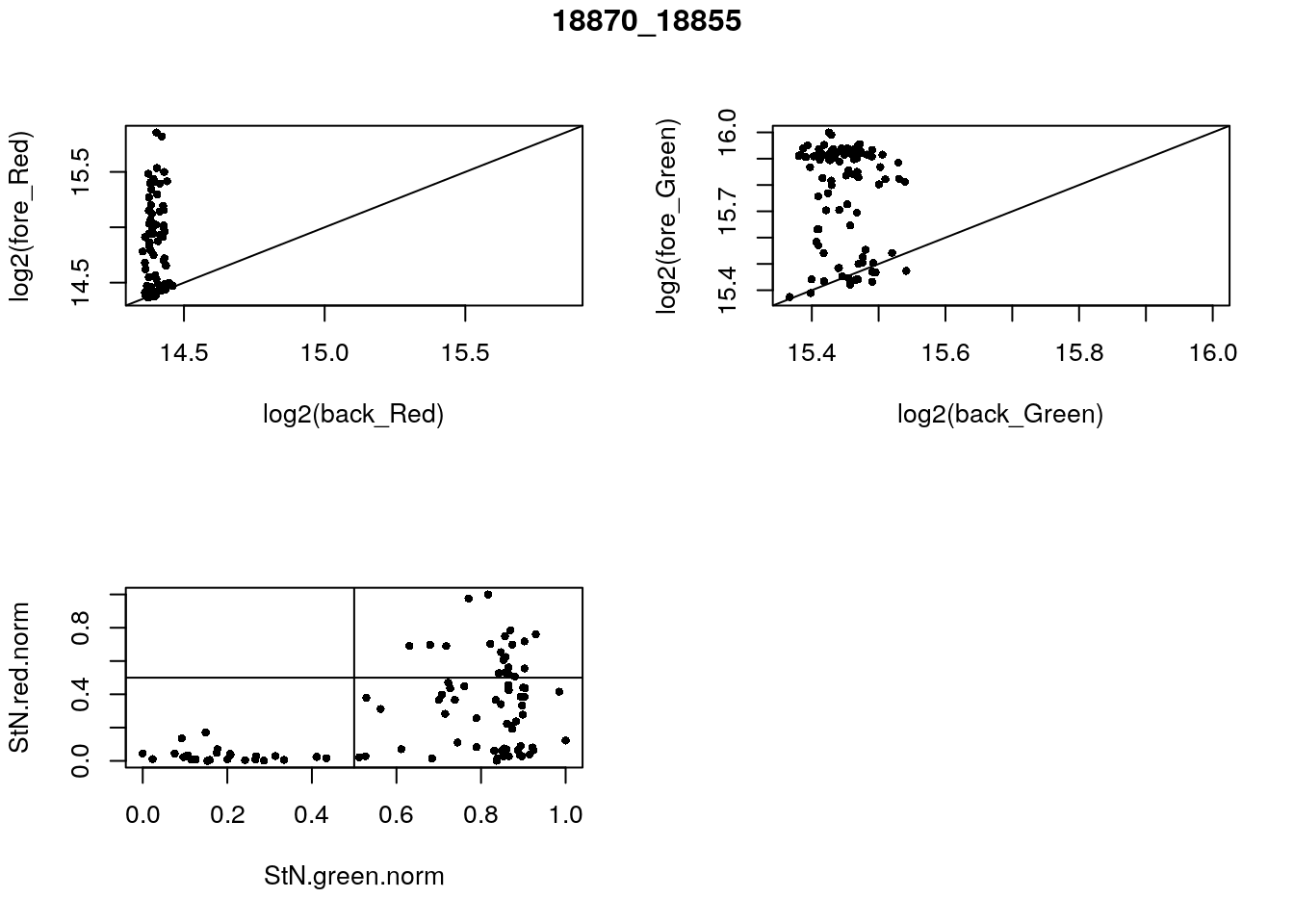
- 18870_19101
eda(confess_18870_19101, "18870_19101")
with(confess_18870_19101, {
    StN.red <- log2(fore_Red) - min(log2(back_Red))
    StN.green <- log2(fore_Green) - min(log2(back_Green))
    StN.red.norm <- (StN.red-min(StN.red))/(max(StN.red)-min(StN.red))
    StN.green.norm <- (StN.green-min(StN.green))/(max(StN.green)-min(StN.green))
    green_pos <- StN.green.norm > .5
    red_pos <- StN.red.norm > .5
    table(red_pos, green_pos)
})
green_pos
red_pos FALSE TRUE
FALSE 33 39
TRUE 0 24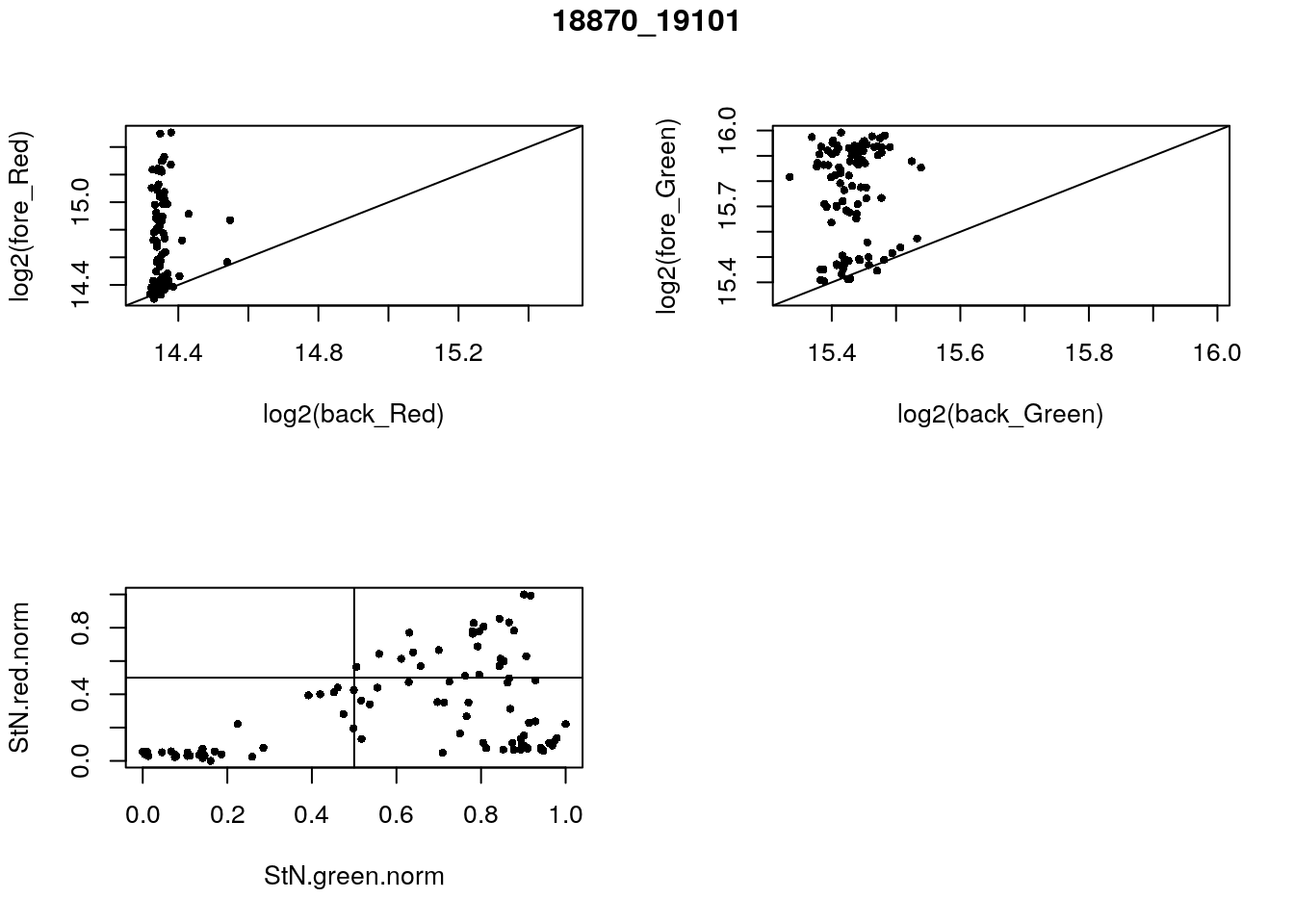
- 19101_19098
eda(confess_19101_19098, "19101_19098")
with(confess_19101_19098, {
    StN.red <- log2(fore_Red) - min(log2(back_Red))
    StN.green <- log2(fore_Green) - min(log2(back_Green))
    StN.red.norm <- (StN.red-min(StN.red))/(max(StN.red)-min(StN.red))
    StN.green.norm <- (StN.green-min(StN.green))/(max(StN.green)-min(StN.green))
    green_pos <- StN.green.norm > .5
    red_pos <- StN.red.norm > .5
    table(red_pos, green_pos)
})
green_pos
red_pos FALSE TRUE
FALSE 32 49
TRUE 0 15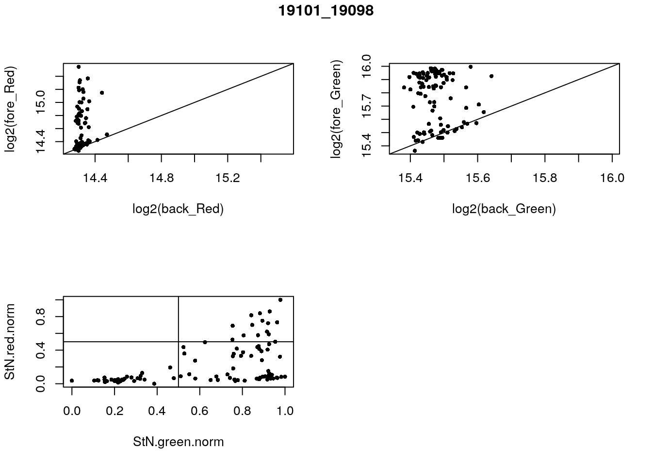
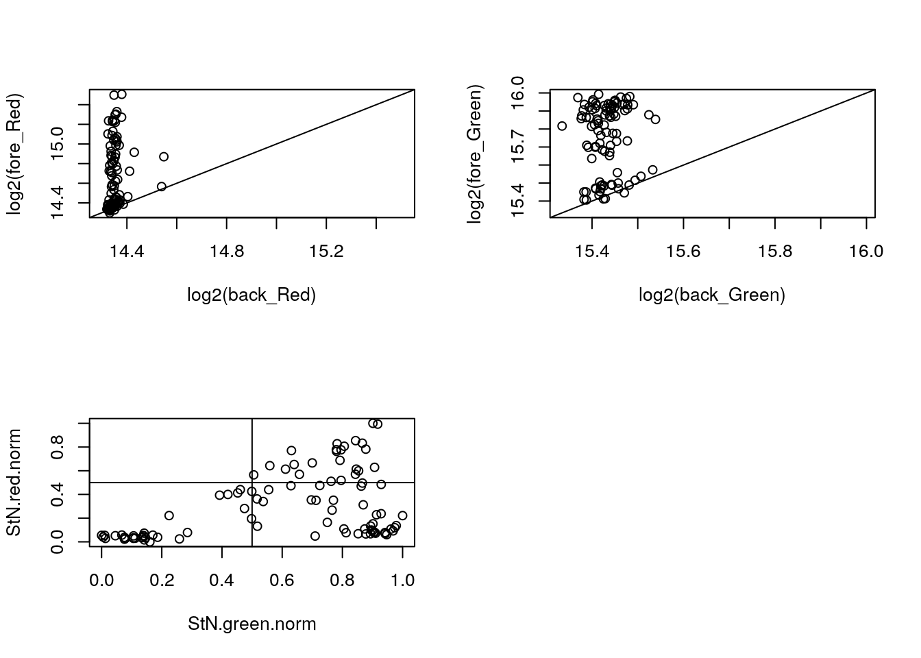
- 18855_18511, crop1
eda(confess_18855_18511_crop1, "18855_18511, crop1")
with(confess_18855_18511_crop1, {
    StN.red <- log2(fore_Red) - min(log2(back_Red))
    StN.green <- log2(fore_Green) - min(log2(back_Green))
    StN.red.norm <- (StN.red-min(StN.red))/(max(StN.red)-min(StN.red))
    StN.green.norm <- (StN.green-min(StN.green))/(max(StN.green)-min(StN.green))
    green_pos <- StN.green.norm > .5
    red_pos <- StN.red.norm > .5
    table(red_pos, green_pos)
})
green_pos
red_pos FALSE TRUE
FALSE 28 46
TRUE 1 21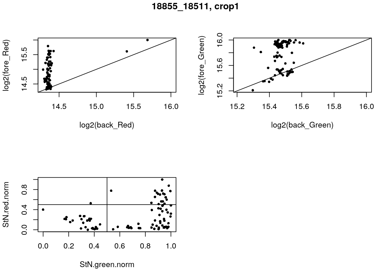
- 18855_18511, crop2
eda(confess_18855_18511_crop2, "18855_18511, crop2")
with(confess_18855_18511_crop2, {
    StN.red <- log2(fore_Red) - min(log2(back_Red))
    StN.green <- log2(fore_Green) - min(log2(back_Green))
    StN.red.norm <- (StN.red-min(StN.red))/(max(StN.red)-min(StN.red))
    StN.green.norm <- (StN.green-min(StN.green))/(max(StN.green)-min(StN.green))
    green_pos <- StN.green.norm > .5
    red_pos <- StN.red.norm > .5
    table(red_pos, green_pos)
})
green_pos
red_pos FALSE TRUE
FALSE 25 47
TRUE 2 22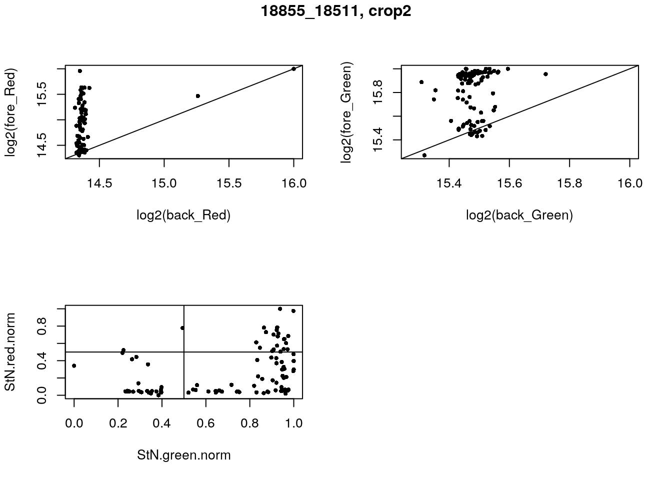
Exploratory analysis
Case 1
Take 18870_18855. Let’s look at the log2fore_red verus log2back_red, which ones are very similar?
with(confess_18870_18855, {
#  xlim_red <- ylim_red <- range(c(log2(back_Red), log2(fore_Red)))
  StN.red <- log2(fore_Red) - min(log2(back_Red))
  StN.green <- log2(fore_Green) - min(log2(back_Green))
  StN.red.norm <- (StN.red-min(StN.red))/(max(StN.red)-min(StN.red))
  StN.green.norm <- (StN.green-min(StN.green))/(max(StN.green)-min(StN.green))

  which_cell <- StN.green.norm < .5 & StN.red.norm < .2

  xy <- cbind(log2(back_Red), log2(fore_Red))
#  xy <- xy[which(abs(log2(fore_Red)-log2(back_Red)) < .05),]
  xy <- xy[which_cell,]
  par(mfrow = c(1,1))
  plot(xy,
       xlim = c(14.35,14.6), ylim = c(14.35,14.6),
       xlab = "log2(Red background)",
       ylab = "log2(Red foreground)",
       pch = 16,
#       pch = as.character(1:96)[which(log(back_Red) < 14.5)],
       cex = .8); abline(0, 1)
})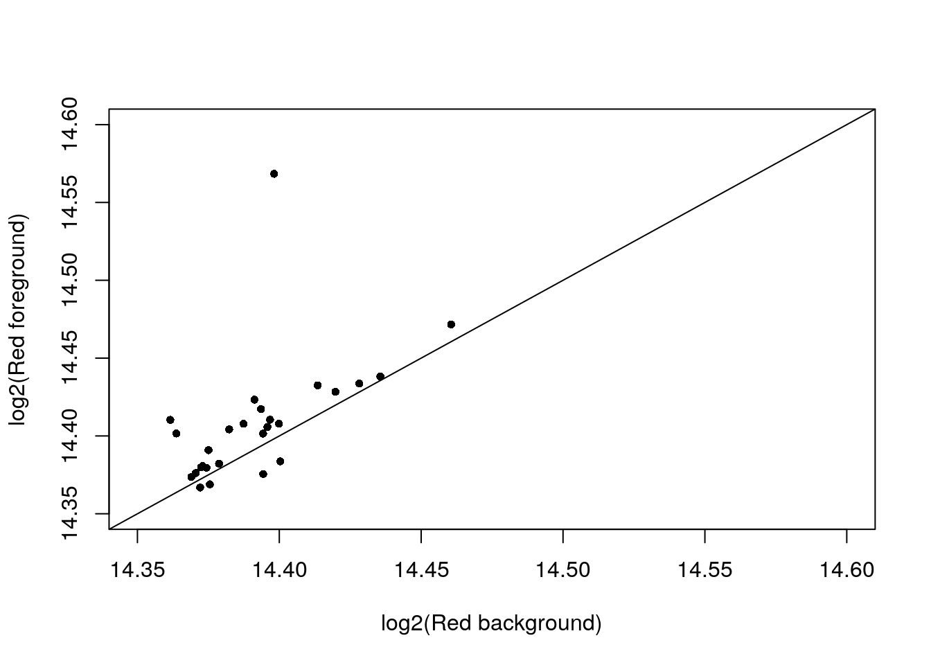
Consider the cells which foreground Red and Background Red are very similar. Of these 28 cells, about half have no DAPI signals and the ones with DAPI signal exhibit green signal.
with(confess_18870_18855, {
     StN.red <- log2(fore_Red) - min(log2(back_Red))
     StN.green <- log2(fore_Green) - min(log2(back_Green))
     StN.red.norm <- (StN.red-min(StN.red))/(max(StN.red)-min(StN.red))
     StN.green.norm <- (StN.green-min(StN.green))/(max(StN.green)-min(StN.green))
     print(which(StN.green.norm < .5 & StN.red.norm < .2))
     })
[1] 14 16 20 21 22 28 30 33 35 39 41 43 44 46 48 49 54 58 60 62 63 64 68
[24] 71 72 74 75 95DAPI/Red/Green 14: Y/N/Y 16: N/N/N 20: ?/N/N 21: Y/N/Y 22: Y/?/Y 28: Y/?/Y 30: Y/N/Y 33: ?/N/Y 35: ?/N/? 39: ?/N/? 41: ?/N/? 43: N/N/? 44: N/?/N 46: Y/N/Y 48: N/N/N 49: N/N/? 54: Y/N/Y 58: Y/?/Y 60: Y/N/Y 62: N/N/N 63: Y/N/Y 64: Y/N/Y 68: N/N/? 71: N/N/? 72: Y/N/Y 74: ?/N/Y 75: Y/Y/Y 95: ?/N/?
Case 2
Consider 18870_19101. Results are similar to 18870_18855.
with(confess_18870_19101, {
xlim_red <- ylim_red <- range(c(log2(back_Red), log2(fore_Red)))
xlim_green <- ylim_green <- range(c(log2(back_Green), log2(fore_Green)))
par(mfrow = c(2,2))
plot(x = log2(back_Red), y = log2(fore_Red),
xlim = xlim_red, ylim = ylim_red); abline(0, 1)
plot(x = log2(back_Green), y = log2(fore_Green),
xlim = xlim_green, ylim = ylim_green); abline(0, 1)
StN.red <- log2(fore_Red) - min(log2(back_Red))
StN.green <- log2(fore_Green) - min(log2(back_Green))
StN.red.norm <- (StN.red-min(StN.red))/(max(StN.red)-min(StN.red))
StN.green.norm <- (StN.green-min(StN.green))/(max(StN.green)-min(StN.green))
plot(x = StN.green.norm,
y = StN.red.norm); abline(v=.5, h = .5)
})
Look at the log2fore_red verus log2back_red, which ones are very similar?
with(confess_18870_19101, {
# xlim_red <- ylim_red <- range(c(log2(back_Red), log2(fore_Red)))
StN.red <- log2(fore_Red) - min(log2(back_Red))
StN.green <- log2(fore_Green) - min(log2(back_Green))
StN.red.norm <- (StN.red-min(StN.red))/(max(StN.red)-min(StN.red))
StN.green.norm <- (StN.green-min(StN.green))/(max(StN.green)-min(StN.green))
which_cell <- StN.green.norm < .3 & StN.red.norm < .3
xy <- cbind(log2(back_Red), log2(fore_Red))
# xy <- xy[which(abs(log2(fore_Red)-log2(back_Red)) < .05),]
xy <- xy[which_cell,]
par(mfrow = c(1,1))
plot(xy,
xlim = c(14.28,14.6), ylim = c(14.28,14.6),
xlab = "log2(Red background)",
ylab = "log2(Red foreground)",
pch = 16,
# pch = as.character(1:96)[which(log(back_Red) < 14.5)],
cex = .8); abline(0, 1)
})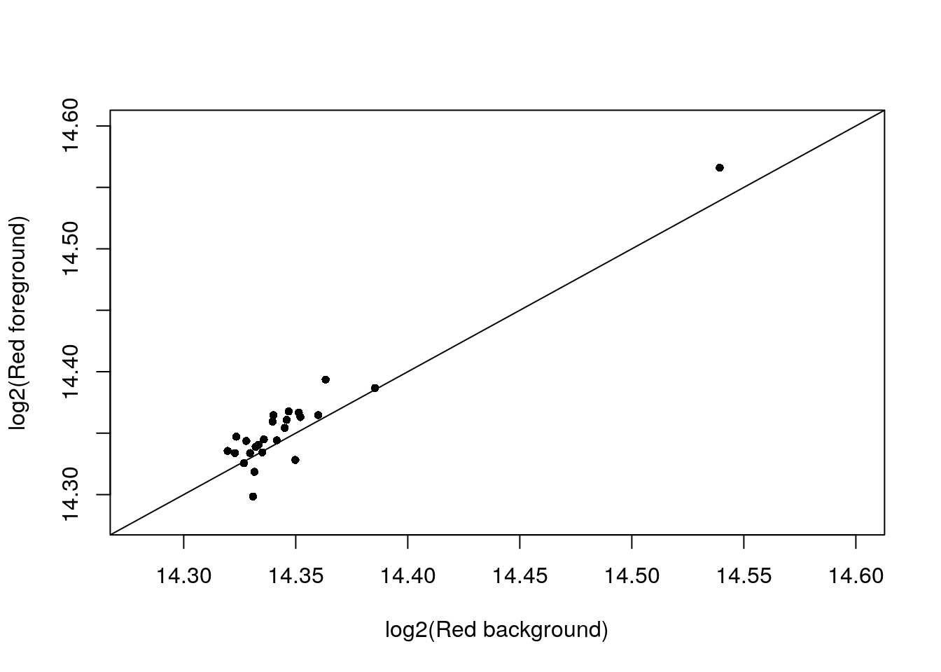
Consider the cells which foreground Red and Background Red are very similar. Of these 28 cells, about half have no DAPI signals and the ones with DAPI signal exhibit green signal.
with(confess_18870_19101, {
StN.red <- log2(fore_Red) - min(log2(back_Red))
StN.green <- log2(fore_Green) - min(log2(back_Green))
StN.red.norm <- (StN.red-min(StN.red))/(max(StN.red)-min(StN.red))
StN.green.norm <- (StN.green-min(StN.green))/(max(StN.green)-min(StN.green))
print(which(StN.green.norm < .3 & StN.red.norm < .3))
}) [1] 2 9 11 12 16 18 21 23 28 30 34 35 36 37 38 45 47 55 61 66 72 73 75
[24] 76 78 87Digging in CONFESS
Observe that 19 out of 28 cells that are called as both Green and Red negative were estimated using BF method. There are other two methods: Both.Channels and One.channel. What’s the difference between these? TBD.
with(confess_18870_18855, {
xlim_red <- ylim_red <- range(c(log2(back_Red), log2(fore_Red)))
xlim_green <- ylim_green <- range(c(log2(back_Green), log2(fore_Green)))
par(mfrow = c(2,2))
plot(x = log2(back_Red), y = log2(fore_Red),
xlim = xlim_red, ylim = ylim_red); abline(0, 1)
plot(x = log2(back_Green), y = log2(fore_Green),
xlim = xlim_green, ylim = ylim_green); abline(0, 1)
StN.red <- log2(fore_Red) - min(log2(back_Red))
StN.green <- log2(fore_Green) - min(log2(back_Green))
StN.red.norm <- (StN.red-min(StN.red))/(max(StN.red)-min(StN.red))
StN.green.norm <- (StN.green-min(StN.green))/(max(StN.green)-min(StN.green))
plot(x = StN.green.norm,
y = StN.red.norm); abline(v=.5, h = .5)
which_cell <- StN.green.norm < .5 & StN.red.norm < .5
print(table(which_cell, Estimation.Type))
print(which(which_cell))
}) Estimation.Type
which_cell BF Both.Channels One.Channel
FALSE 1 46 21
TRUE 19 4 5
 [1] 14 16 20 21 22 28 30 33 35 39 41 43 44 46 48 49 54 58 60 62 63 64 68
[24] 71 72 74 75 95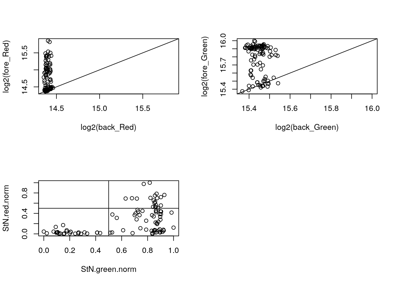
Session information
sessionInfo()R version 3.4.2 (2017-09-28)
Platform: x86_64-pc-linux-gnu (64-bit)
Running under: Ubuntu 17.04
Matrix products: default
BLAS: /usr/lib/libblas/libblas.so.3.7.0
LAPACK: /usr/lib/lapack/liblapack.so.3.7.0
locale:
[1] LC_CTYPE=en_US.UTF-8 LC_NUMERIC=C
[3] LC_TIME=en_US.UTF-8 LC_COLLATE=en_US.UTF-8
[5] LC_MONETARY=en_US.UTF-8 LC_MESSAGES=en_US.UTF-8
[7] LC_PAPER=en_US.UTF-8 LC_NAME=C
[9] LC_ADDRESS=C LC_TELEPHONE=C
[11] LC_MEASUREMENT=en_US.UTF-8 LC_IDENTIFICATION=C
attached base packages:
[1] stats graphics grDevices utils datasets methods base
loaded via a namespace (and not attached):
[1] compiler_3.4.2 backports_1.1.1 magrittr_1.5 rprojroot_1.2
[5] tools_3.4.2 htmltools_0.3.6 yaml_2.1.14 Rcpp_0.12.11
[9] stringi_1.1.5 rmarkdown_1.6 knitr_1.17 git2r_0.19.0
[13] stringr_1.2.0 digest_0.6.12 evaluate_0.10.1Session information
sessionInfo()R version 3.4.2 (2017-09-28)
Platform: x86_64-pc-linux-gnu (64-bit)
Running under: Ubuntu 17.04
Matrix products: default
BLAS: /usr/lib/libblas/libblas.so.3.7.0
LAPACK: /usr/lib/lapack/liblapack.so.3.7.0
locale:
[1] LC_CTYPE=en_US.UTF-8 LC_NUMERIC=C
[3] LC_TIME=en_US.UTF-8 LC_COLLATE=en_US.UTF-8
[5] LC_MONETARY=en_US.UTF-8 LC_MESSAGES=en_US.UTF-8
[7] LC_PAPER=en_US.UTF-8 LC_NAME=C
[9] LC_ADDRESS=C LC_TELEPHONE=C
[11] LC_MEASUREMENT=en_US.UTF-8 LC_IDENTIFICATION=C
attached base packages:
[1] stats graphics grDevices utils datasets methods base
loaded via a namespace (and not attached):
[1] compiler_3.4.2 backports_1.1.1 magrittr_1.5 rprojroot_1.2
[5] tools_3.4.2 htmltools_0.3.6 yaml_2.1.14 Rcpp_0.12.11
[9] stringi_1.1.5 rmarkdown_1.6 knitr_1.17 git2r_0.19.0
[13] stringr_1.2.0 digest_0.6.12 evaluate_0.10.1This R Markdown site was created with workflowr