Sample QC
Po-Yuan Tung
2017-11-28
Last updated: 2018-02-06
Code version: fd3bf7b
Setup
library("cowplot")
library("dplyr")
library("edgeR")
library("ggplot2")
library("reshape2")
library("Biobase")
source("../code/pca.R")
theme_set(cowplot::theme_cowplot())

# The palette with grey:
cbPalette <- c("#999999", "#E69F00", "#56B4E9", "#009E73", "#F0E442", "#0072B2", "#D55E00", "#CC79A7")
fname <- Sys.glob("../data/eset/*.rds")
eset <- Reduce(combine, Map(readRDS, fname))
anno <- pData(eset)Total mapped reads
Note: Using the 15% cutoff of samples with no cells excludes all the samples
## calculate the cut-off
cut_off_reads <- quantile(anno[anno$cell_number == 0,"mapped"], 0.85)

cut_off_reads
85%
733229.6 anno$cut_off_reads <- anno$mapped > cut_off_reads
## numbers of cells
sum(anno[anno$cell_number == 1, "mapped"] > cut_off_reads)[1] 1146sum(anno[anno$cell_number == 1, "mapped"] <= cut_off_reads)[1] 161## density plots
plot_reads <- ggplot(anno[anno$cell_number == 0 |
anno$cell_number == 1 , ],
aes(x = mapped, fill = as.factor(cell_number))) +
geom_density(alpha = 0.5) +
geom_vline(xintercept = cut_off_reads, colour="grey", linetype = "longdash") +
labs(x = "Total mapped reads", title = "Number of total mapped reads", fill = "Cell number")
plot_reads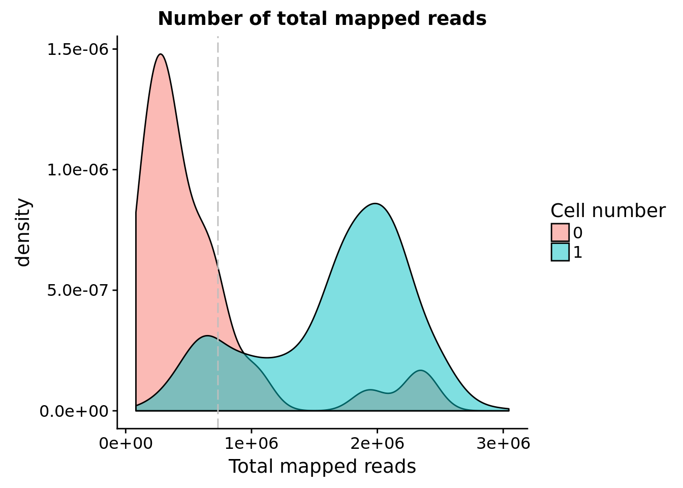
Unmapped ratios
Note: Using the 30 % cutoff of samples with no cells excludes all the samples
## calculate unmapped ratios
anno$unmapped_ratios <- anno$unmapped/anno$umi

## cut off
cut_off_unmapped <- quantile(anno[anno$cell_number == 0,"unmapped_ratios"], 0.3)

cut_off_unmapped
30%
0.4216077 anno$cut_off_unmapped <- anno$unmapped_ratios < cut_off_unmapped
## numbers of cells
sum(anno[anno$cell_number == 1, "unmapped_ratios"] >= cut_off_unmapped)[1] 254sum(anno[anno$cell_number == 1, "unmapped_ratios"] < cut_off_unmapped)[1] 1053## density plots
plot_unmapped <- ggplot(anno[anno$cell_number == 0 |
anno$cell_number == 1 , ],
aes(x = unmapped_ratios *100, fill = as.factor(cell_number))) +
geom_density(alpha = 0.5) +
geom_vline(xintercept = cut_off_unmapped *100, colour="grey", linetype = "longdash") +
labs(x = "Unmapped reads/ total reads", title = "Unmapped reads percentage")
plot_unmapped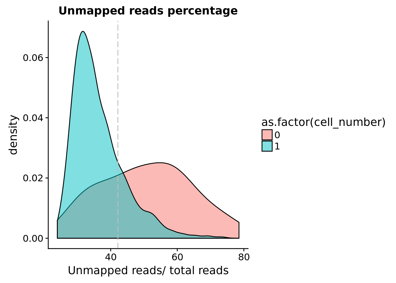 Look at the unmapped percentage per sample by C1 experimnet and by individual.
unmapped_exp <- ggplot(anno, aes(x = as.factor(experiment), y = unmapped_ratios, color = as.factor(experiment))) +
  geom_violin() +
  geom_boxplot(alpha = .01, width = .2, position = position_dodge(width = .9)) +
  labs(x = "C1 chip", y = "Unmapped reads/ total reads",
       title = "Unmapped reads percentage") +
  theme(legend.title = element_blank(),
        axis.text.x = element_text(angle = 45, hjust = 1, vjust = 1))

unmapped_indi <- ggplot(anno, aes(x = chip_id, y = unmapped_ratios, color = as.factor(chip_id))) +
  geom_violin() +
  geom_boxplot(alpha = .01, width = .2, position = position_dodge(width = .9)) +
  labs(x = "C1 chip", y = "Unmapped reads/ total reads",
       title = "Unmapped reads percentage") +
  theme(legend.title = element_blank(),
        axis.text.x = element_text(angle = 45, hjust = 1, vjust = 1))

plot_grid(unmapped_exp + theme(legend.position = "none"),
          unmapped_indi + theme(legend.position = "none"),
          labels = letters[1:2])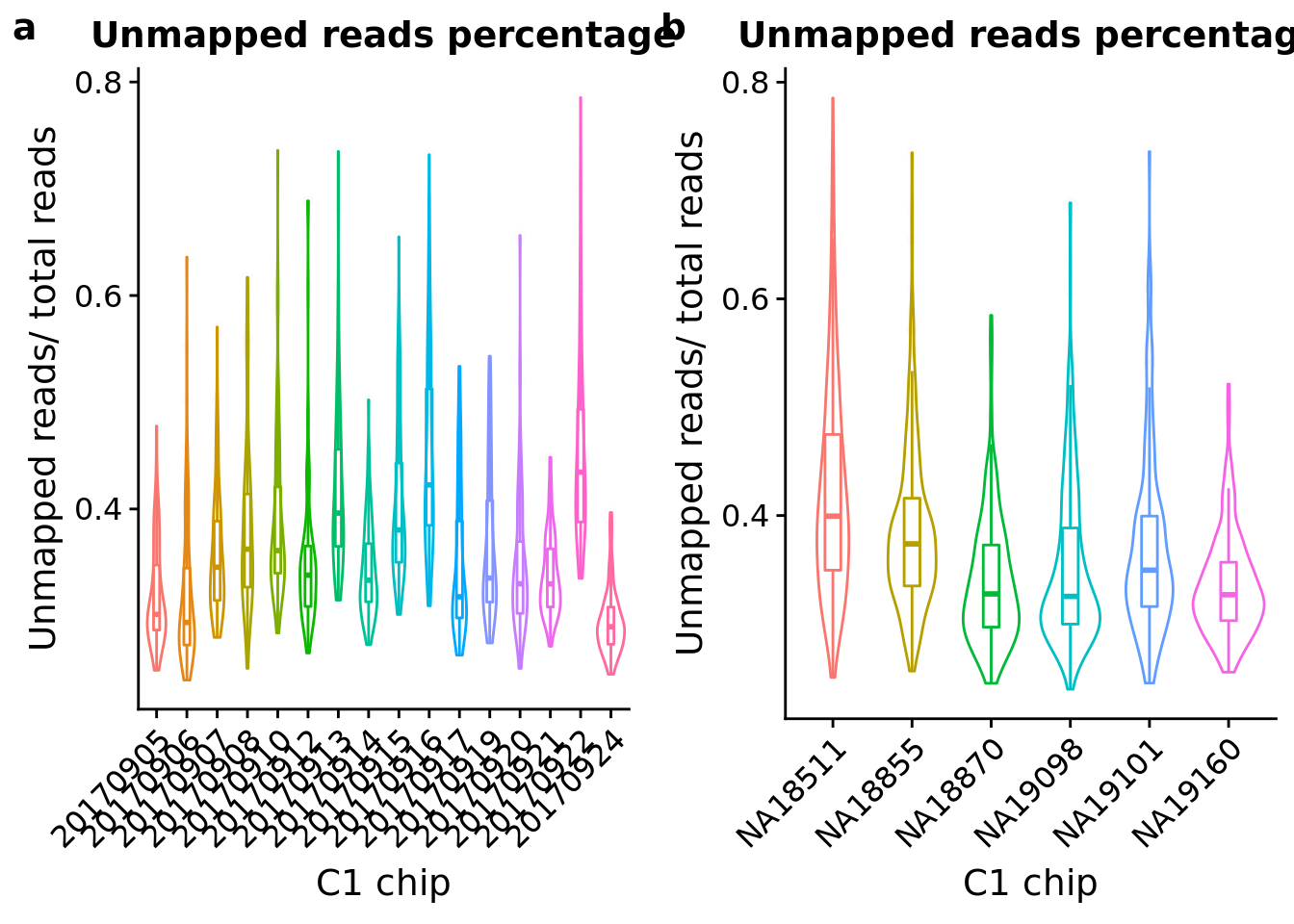
ERCC percentage
## calculate ercc reads percentage
anno$ercc_percentage <- anno$reads_ercc / anno$mapped

## cut off
cut_off_ercc <- quantile(anno[anno$cell_number == 0,"ercc_percentage"], 0.15)

cut_off_ercc
15%
0.1673614 anno$cut_off_ercc <- anno$ercc_percentage < cut_off_ercc
## numbers of cells
sum(anno[anno$cell_number == 1, "ercc_percentage"] >= cut_off_ercc)[1] 225sum(anno[anno$cell_number == 1, "ercc_percentage"] < cut_off_ercc)[1] 1082## density plots
plot_ercc <- ggplot(anno[anno$cell_number == 0 |
anno$cell_number == 1 , ],
aes(x = ercc_percentage *100, fill = as.factor(cell_number))) +
geom_density(alpha = 0.5) +
geom_vline(xintercept = cut_off_ercc *100, colour="grey", linetype = "longdash") +
labs(x = "ERCC reads / total mapped reads", title = "ERCC reads percentage")
plot_ercc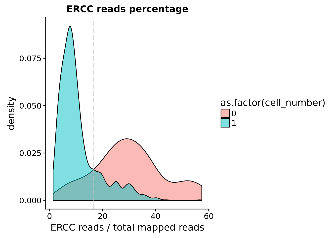
Look at the ERCC spike-in percentage per sample by C1 experimnet and by individual.
ercc_exp <- ggplot(anno, aes(x = as.factor(experiment), y = ercc_percentage, color = as.factor(experiment))) +
  geom_violin() +
  geom_boxplot(alpha = .01, width = .2, position = position_dodge(width = .9)) +
  labs(x = "C1 chip", y = "ERCC percentage",
       title = "ERCC percentage per sample") +
  theme(legend.title = element_blank(),
        axis.text.x = element_text(angle = 45, hjust = 1, vjust = 1))

ercc_indi <- ggplot(anno, aes(x = chip_id, y = ercc_percentage, color = as.factor(chip_id))) +
  geom_violin() +
  geom_boxplot(alpha = .01, width = .2, position = position_dodge(width = .9)) +
  labs(x = "C1 chip", y = "ERCC percentage",
       title = "ERCC percentage per sample") +
  theme(legend.title = element_blank(),
        axis.text.x = element_text(angle = 45, hjust = 1, vjust = 1))

plot_grid(ercc_exp + theme(legend.position = "none"),
          ercc_indi + theme(legend.position = "none"),
          labels = letters[1:2])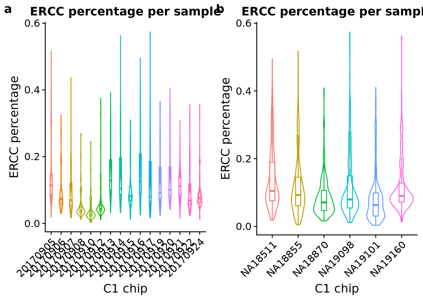
Number of genes detected
## cut off
cut_off_genes <- quantile(anno[anno$cell_number == 0,"detect_hs"], 0.85)

cut_off_genes
85%
5901.4 anno$cut_off_genes <- anno$detect_hs > cut_off_genes
## numbers of cells
sum(anno[anno$cell_number == 1, "detect_hs"] > cut_off_genes)[1] 1079sum(anno[anno$cell_number == 1, "detect_hs"] <= cut_off_genes)[1] 228## density plots
plot_gene <- ggplot(anno[anno$cell_number == 0 |
anno$cell_number == 1 , ],
aes(x = detect_hs, fill = as.factor(cell_number))) +
geom_density(alpha = 0.5) +
geom_vline(xintercept = cut_off_genes, colour="grey", linetype = "longdash") +
labs(x = "Gene numbers", title = "Numbers of detected genes")
plot_gene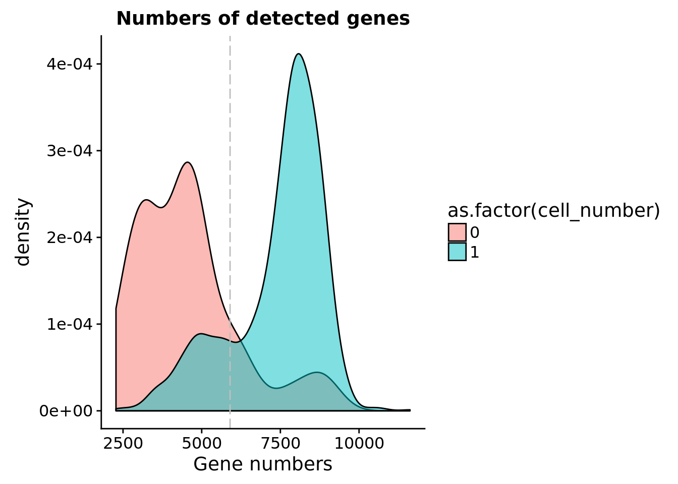
number_exp <- ggplot(anno, aes(x = as.factor(experiment), y = detect_hs, color = as.factor(experiment))) +
  geom_violin() +
  geom_boxplot(alpha = .01, width = .2, position = position_dodge(width = .9)) +
  labs(x = "C1 chip", y = "Number of genes detected",
       title = "Number of genes per sample") +
  theme(legend.title = element_blank(),
        axis.text.x = element_text(angle = 45, hjust = 1, vjust = 1))

number_indi <- ggplot(anno, aes(x = chip_id, y = detect_hs, color = as.factor(chip_id))) +
  geom_violin() +
  geom_boxplot(alpha = .01, width = .2, position = position_dodge(width = .9)) +
  labs(x = "C1 chip", y = "Number of genes detected",
       title = "Number of genes per sample") +
  theme(legend.title = element_blank(),
        axis.text.x = element_text(angle = 45, hjust = 1, vjust = 1))

plot_grid(number_exp + theme(legend.position = "none"),
          number_indi + theme(legend.position = "none"),
          labels = letters[1:2])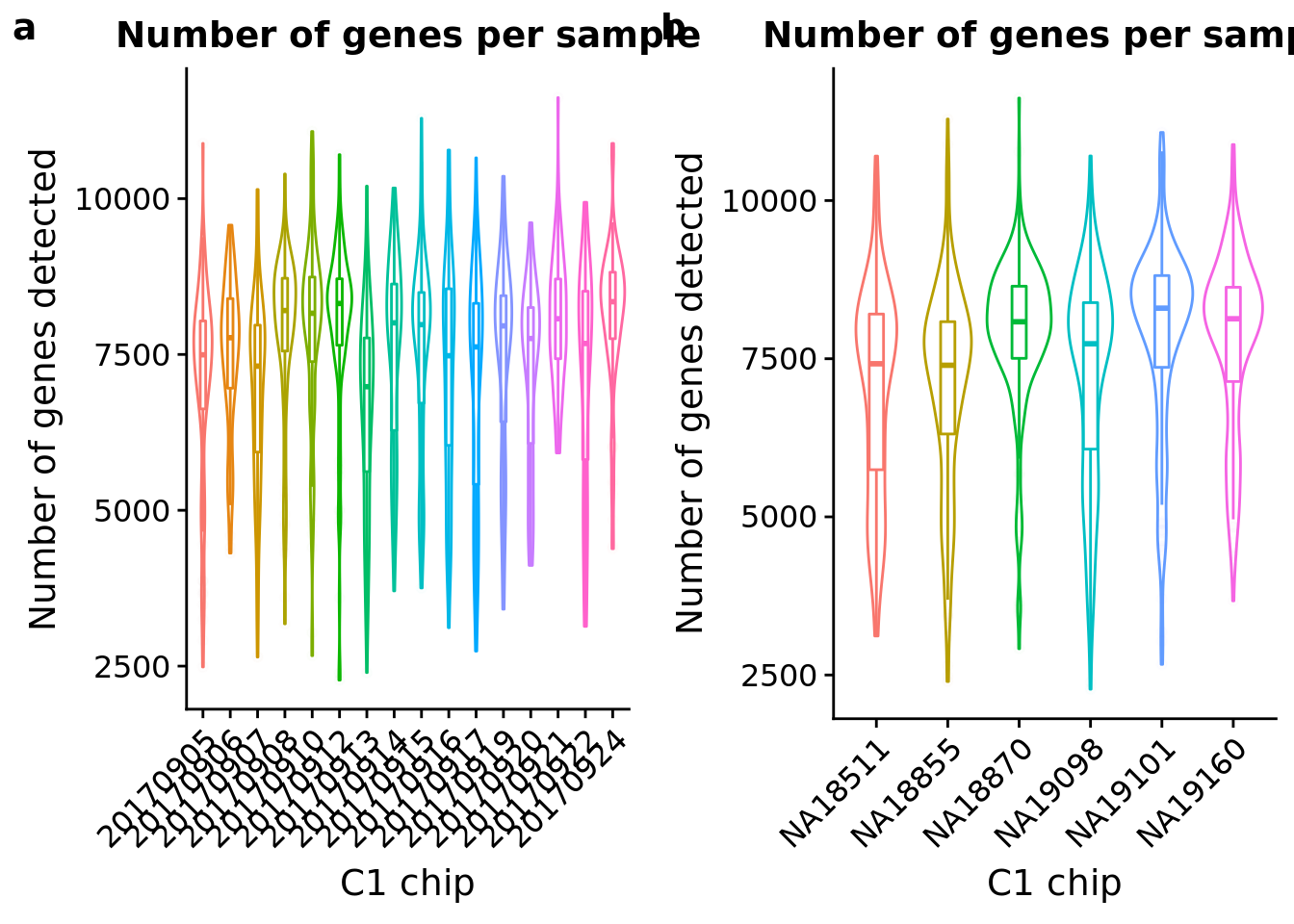
FUCCI transgene
## plot molecule number of egfp and mCherry
egfp_mol <- ggplot(anno[anno$cell_number == 0 |
            anno$cell_number == 1 , ],
       aes(x = mol_egfp, fill = as.factor(cell_number))) +
       geom_density(alpha = 0.5) +
       labs(x = "EGFP molecule numbers", title = "Numbers of EGFP molecules")

mcherry_mol <- ggplot(anno[anno$cell_number == 0 |
            anno$cell_number == 1 , ],
       aes(x = mol_mcherry, fill = as.factor(cell_number))) +
       geom_density(alpha = 0.5) +
       labs(x = "mCherry molecule numbers", title = "Numbers of mCherry molecules")

plot_grid(egfp_mol + theme(legend.position = c(.5,.9)),
          mcherry_mol + theme(legend.position = "none"),
          labels = letters[1:2])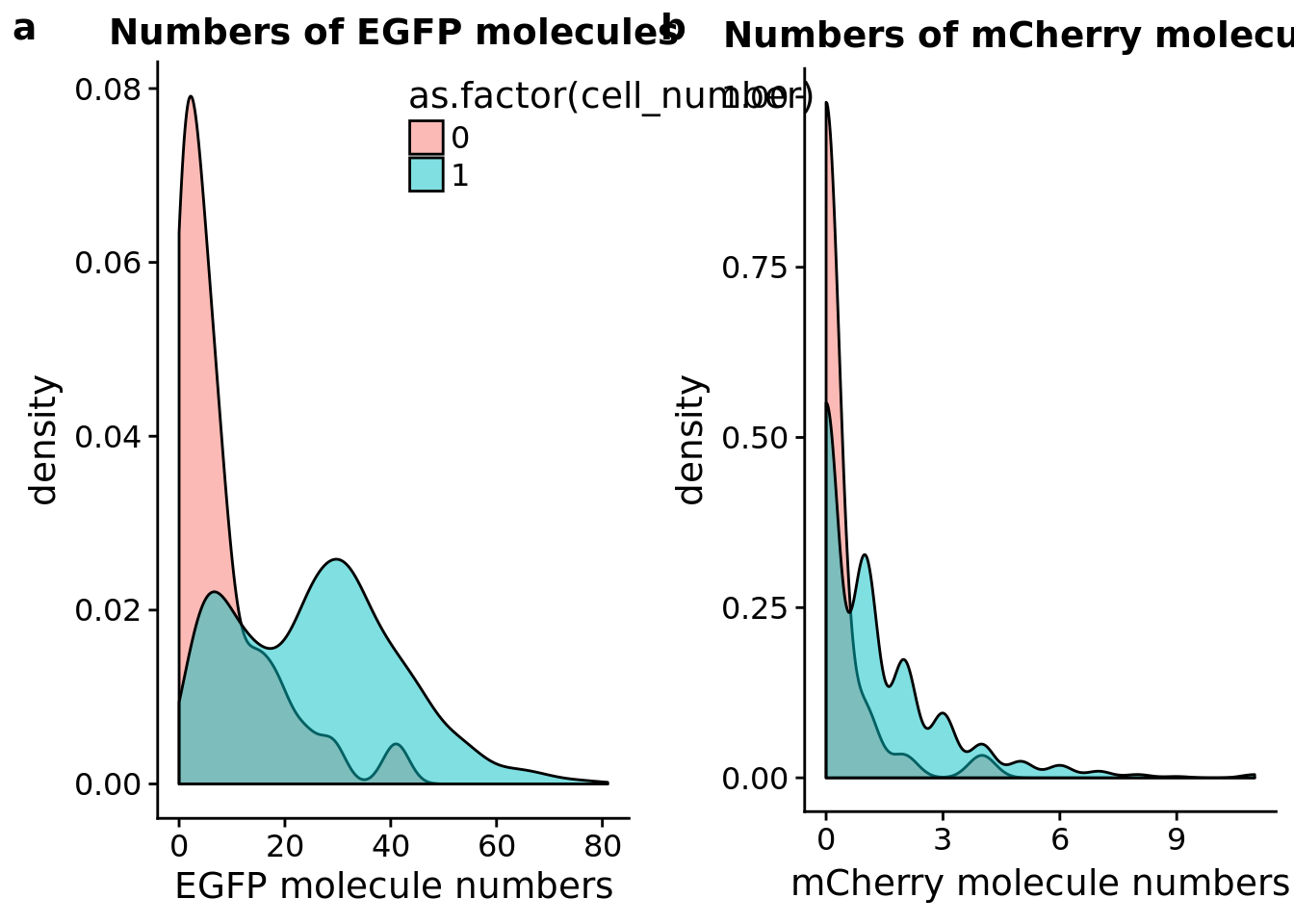
Linear Discriminat Analysis
Total molecule vs concentration
library(MASS)
Attaching package: 'MASS'The following object is masked from 'package:dplyr':
select## create 3 groups according to cell number
group_3 <- rep("two",dim(anno)[1])
group_3[grep("0", anno$cell_number)] <- "no"
group_3[grep("1", anno$cell_number)] <- "one"
## create data frame
data <- anno %>% dplyr::select(experiment:concentration, mapped, molecules)
data <- data.frame(data, group = group_3)
## perform lda
data_lda <- lda(group ~ concentration + molecules, data = data)
data_lda_p <- predict(data_lda, newdata = data[,c("concentration", "molecules")])$class
## determine how well the model fix
table(data_lda_p, data[, "group"])
data_lda_p   no  one  two
       no     0    0    0
       one   36 1297  147
       two    0   11   45
data$data_lda_p <- data_lda_p
## plot before and after
plot_before <- ggplot(data, aes(x = concentration, y = molecules / 10^3,
color = as.factor(group))) +
geom_text(aes(label = cell_number, alpha = 0.5)) +
labs(x = "Concentration", y = "Gene molecules (thousands)", title = "Before") +
scale_color_brewer(palette = "Dark2") +
theme(legend.position = "none")
plot_after <- ggplot(data, aes(x = concentration, y = molecules / 10^3,
color = as.factor(data_lda_p))) +
geom_text(aes(label = cell_number, alpha = 0.5)) +
labs(x = "Concentration", y = "Gene molecules (thousands)", title = "After") +
scale_color_brewer(palette = "Dark2") +
theme(legend.position = "none")
plot_grid(plot_before + theme(legend.position=c(.8,.85)),
plot_after + theme(legend.position = "none"),
labels = LETTERS[1:2])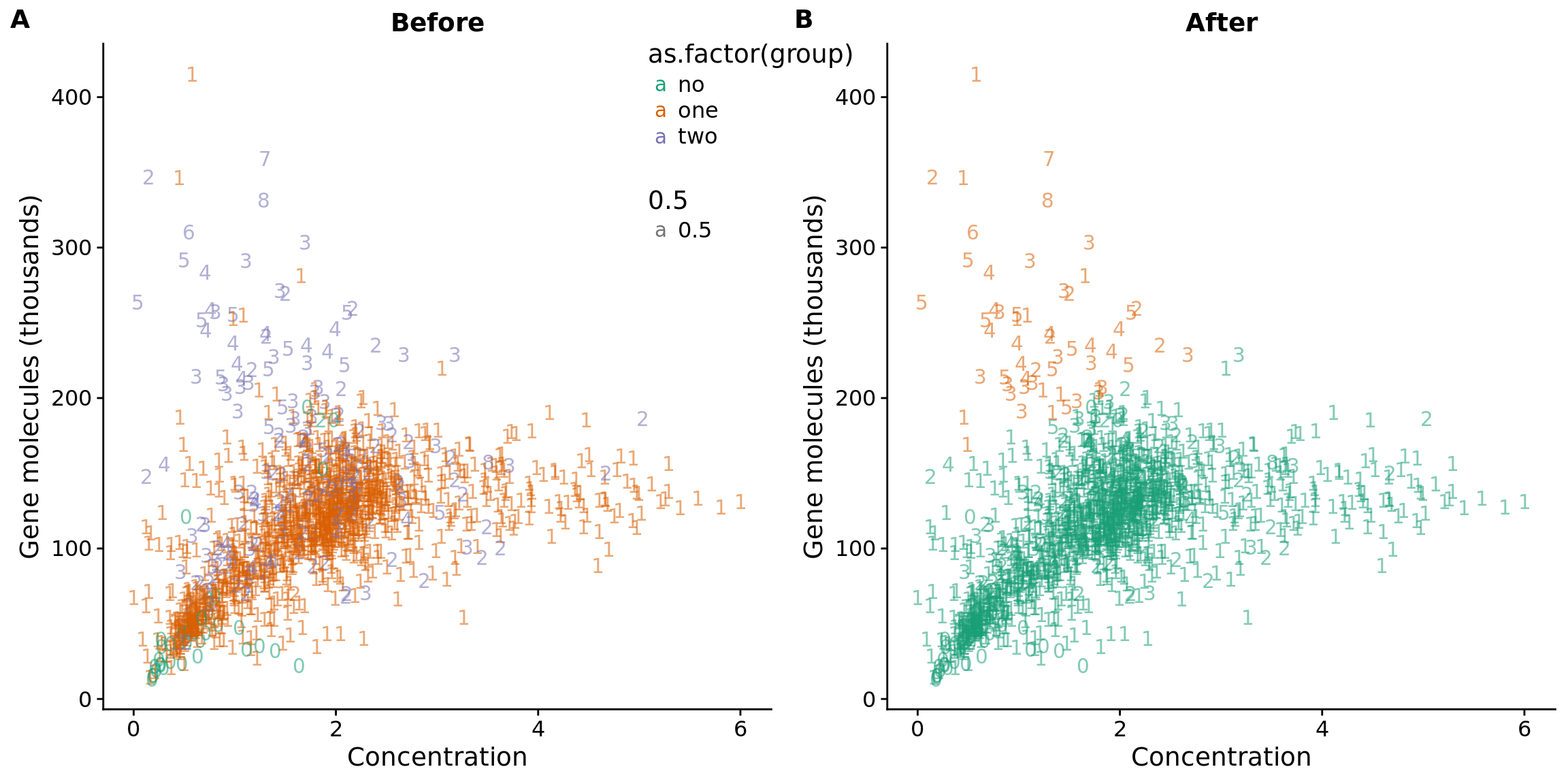
Reads to molecule conversion
## calculate convertion
anno$ercc_conversion <- anno$mol_ercc / anno$reads_ercc

anno$conversion <- anno$mol_hs / anno$reads_hs

## try lda
data$conversion <- anno$conversion
data$ercc_conversion <- anno$ercc_conversion

data_ercc_lda <- lda(group ~ ercc_conversion + conversion, data = data)

data_ercc_lda_p <- predict(data_ercc_lda,  newdata = data[,c("ercc_conversion", "conversion")])$class

## determine how well the model fix
table(data_ercc_lda_p, data[, "group"])
data_ercc_lda_p   no  one  two
            no    15   29    1
            one   21 1275  165
            two    0    4   26
data$data_ercc_lda_p <- data_ercc_lda_p
## cutoff
#out_ercc_con <- anno %>% filter(cell_number == "1", ercc_conversion > .094)
anno$conversion_outlier <- anno$cell_number == 1 & anno$ercc_conversion > .094
## plot before and after
plot_ercc_before <- ggplot(data, aes(x = ercc_conversion, y = conversion,
color = as.factor(group))) +
geom_text(aes(label = cell_number, alpha = 0.5)) +
labs(x = "Convertion of ERCC spike-ins", y = "Conversion of genes", title = "Before") +
scale_color_brewer(palette = "Dark2") +
theme(legend.position = "none")
plot_ercc_after <- ggplot(data, aes(x = ercc_conversion, y = conversion,
color = as.factor(data_ercc_lda_p))) +
geom_text(aes(label = cell_number, alpha = 0.5)) +
labs(x = "Convertion of ERCC spike-ins", y = "Conversion of genes", title = "After") +
scale_color_brewer(palette = "Dark2") +
theme(legend.position = "none")
plot_grid(plot_ercc_before,
plot_ercc_after,
labels = LETTERS[3:4])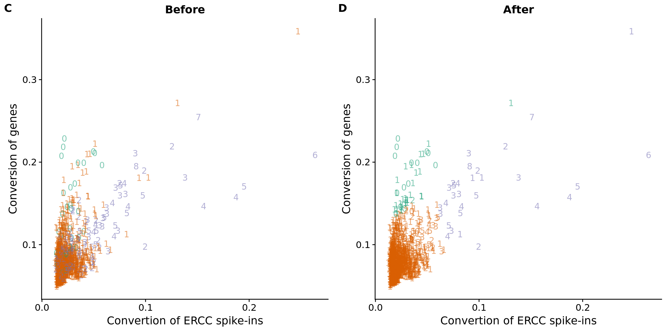
PCA
## look at human genes
eset_hs <- eset[fData(eset)$source == "H. sapiens", ]
head(featureNames(eset_hs))
[1] "ENSG00000000003" "ENSG00000000005" "ENSG00000000419" "ENSG00000000457"
[5] "ENSG00000000460" "ENSG00000000938"## remove genes of all 0s
eset_hs_clean <- eset_hs[rowSums(exprs(eset_hs)) != 0, ]
dim(eset_hs_clean)Features Samples
19348 1536 ## convert to log2 cpm
mol_hs_cpm <- cpm(exprs(eset_hs_clean), log = TRUE)
mol_hs_cpm_means <- rowMeans(mol_hs_cpm)
summary(mol_hs_cpm_means) Min. 1st Qu. Median Mean 3rd Qu. Max.
2.413 2.482 3.180 3.858 4.761 12.999 mol_hs_cpm <- mol_hs_cpm[mol_hs_cpm_means > median(mol_hs_cpm_means), ]
dim(mol_hs_cpm)[1] 9674 1536## pca of genes with reasonable expression levels
pca_hs <- run_pca(mol_hs_cpm)
plot_pca_id <- plot_pca(pca_hs$PCs, pcx = 1, pcy = 2, explained = pca_hs$explained,
metadata = pData(eset_hs_clean), color = "chip_id")Filter
Final list
## all filter
anno$filter_all <- anno$cell_number == 1 &
                   anno$mol_egfp > 0 &
                   anno$valid_id &
                   anno$cut_off_reads &
                   ## anno$cut_off_unmapped &
                   anno$cut_off_ercc &
                   anno$cut_off_genes
sort(table(anno[anno$filter_all, "chip_id"]))
NA18511 NA19160 NA19101 NA18855 NA19098 NA18870
    131     133     142     198     202     227
table(anno[anno$filter_all, c("experiment","chip_id")]) chip_id
experiment NA18511 NA18855 NA18870 NA19098 NA19101 NA19160
20170905 0 38 31 0 0 0
20170906 0 0 0 48 24 0
20170907 0 33 0 26 0 0
20170908 0 0 38 0 38 0
20170910 0 38 0 0 27 0
20170912 0 0 43 39 0 0
20170913 0 50 0 0 0 10
20170914 0 0 0 0 27 36
20170915 27 39 0 0 0 0
20170916 20 0 0 0 26 0
20170917 0 0 0 43 0 12
20170919 12 0 0 46 0 0
20170920 41 0 0 0 0 18
20170921 0 0 46 0 0 26
20170922 31 0 30 0 0 0
20170924 0 0 39 0 0 31Plots
genes_unmapped <-  ggplot(anno,
                   aes(x = detect_hs, y = unmapped_ratios * 100,
                       col = as.factor(chip_id),
                       label = as.character(cell_number),
                       height = 600, width = 2000)) +
                   scale_colour_manual(values=cbPalette) +
                   geom_text(fontface = 3, alpha = 0.5) +
                   geom_vline(xintercept = cut_off_genes,
                              colour="grey", linetype = "longdash") +
                   geom_hline(yintercept = cut_off_unmapped * 100,
                              colour="grey", linetype = "longdash") +
                   labs(x = "Number of detected genes / sample",
                        y = "Percentage of unmapped reads (%)")

genes_spike <- ggplot(anno,
               aes(x = detect_hs, y = ercc_percentage * 100,
                   col = as.factor(chip_id),
                   label = as.character(cell_number),
                   height = 600, width = 2000)) +
               scale_colour_manual(values=cbPalette) +
               scale_shape_manual(values=c(1:10)) +
               geom_text(fontface = 3, alpha = 0.5) +
               geom_vline(xintercept = cut_off_genes,
                          colour="grey", linetype = "longdash") +
               geom_hline(yintercept = cut_off_ercc * 100,
                          colour="grey", linetype = "longdash") +
               labs(x = "Number of detected genes / samlpe",
                    y = "Percentage of ERCC spike-in reads (%)")

reads_unmapped_num <-  ggplot(anno,
                       aes(x = mapped, y = unmapped_ratios * 100,
                           col = as.factor(experiment),
                           label = as.character(cell_number),
                           height = 600, width = 2000)) +
                       geom_text(fontface = 3, alpha = 0.5) +
                       geom_vline(xintercept = cut_off_reads,
                                  colour="grey", linetype = "longdash") +
                       geom_hline(yintercept = cut_off_unmapped * 100,
                                  colour="grey", linetype = "longdash") +
                       labs(x = "Total mapped reads / sample",
                            y = "Percentage of unmapped reads (%)")

reads_spike_num <- ggplot(anno,
                   aes(x = mapped, y = ercc_percentage * 100,
                       col = as.factor(experiment),
                       label = as.character(cell_number),
                       height = 600, width = 2000)) +
                   geom_text(fontface = 3, alpha = 0.5) +
                   geom_vline(xintercept = cut_off_reads,
                              colour="grey", linetype = "longdash") +
                   geom_hline(yintercept = cut_off_ercc * 100,
                              colour="grey", linetype = "longdash") +
                   labs(x = "Total mapped reads / sample",
                        y = "Percentage of ERCC spike-in reads (%)")

plot_grid(genes_unmapped + theme(legend.position = c(.7,.9)),
          genes_spike + theme(legend.position = "none"),
          labels = letters[1:2])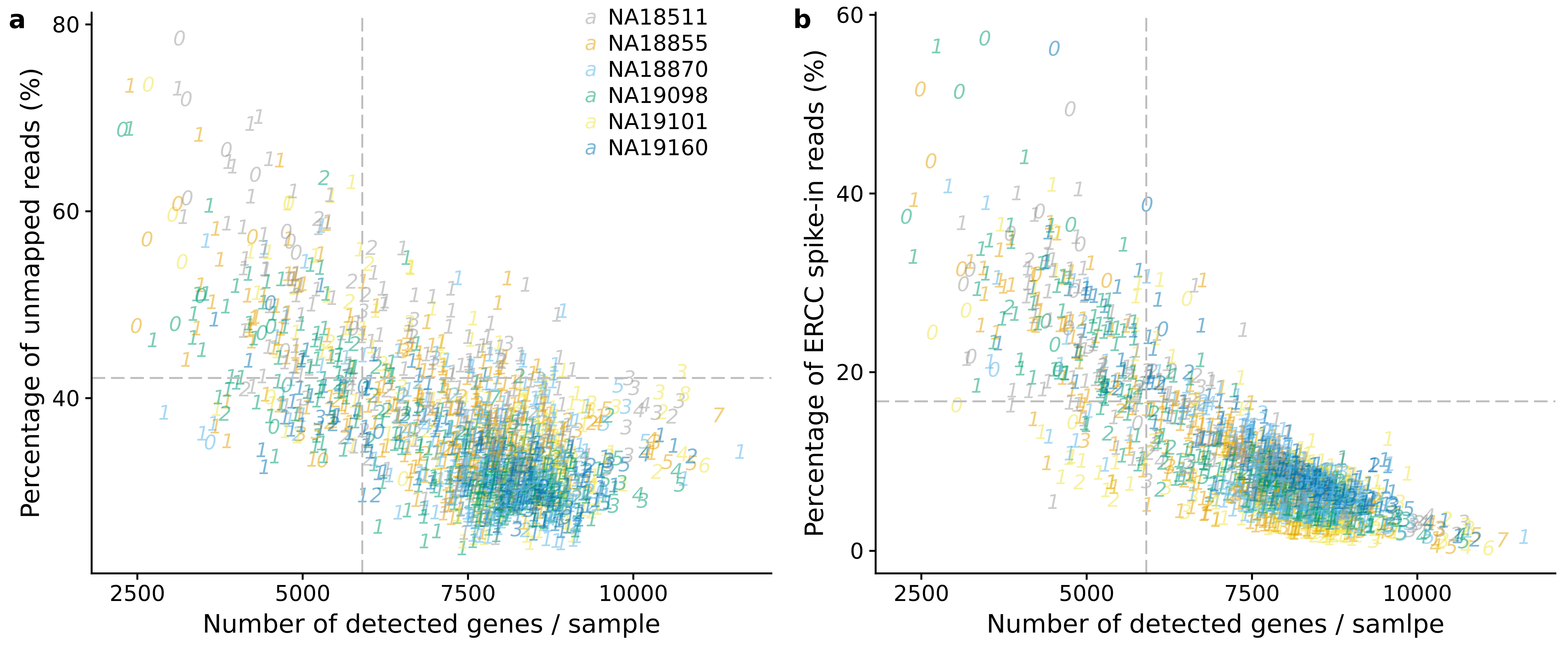
plot_grid(reads_unmapped_num + theme(legend.position = c(.7,.9)),
          reads_spike_num + theme(legend.position = "none"),
          labels = letters[3:4])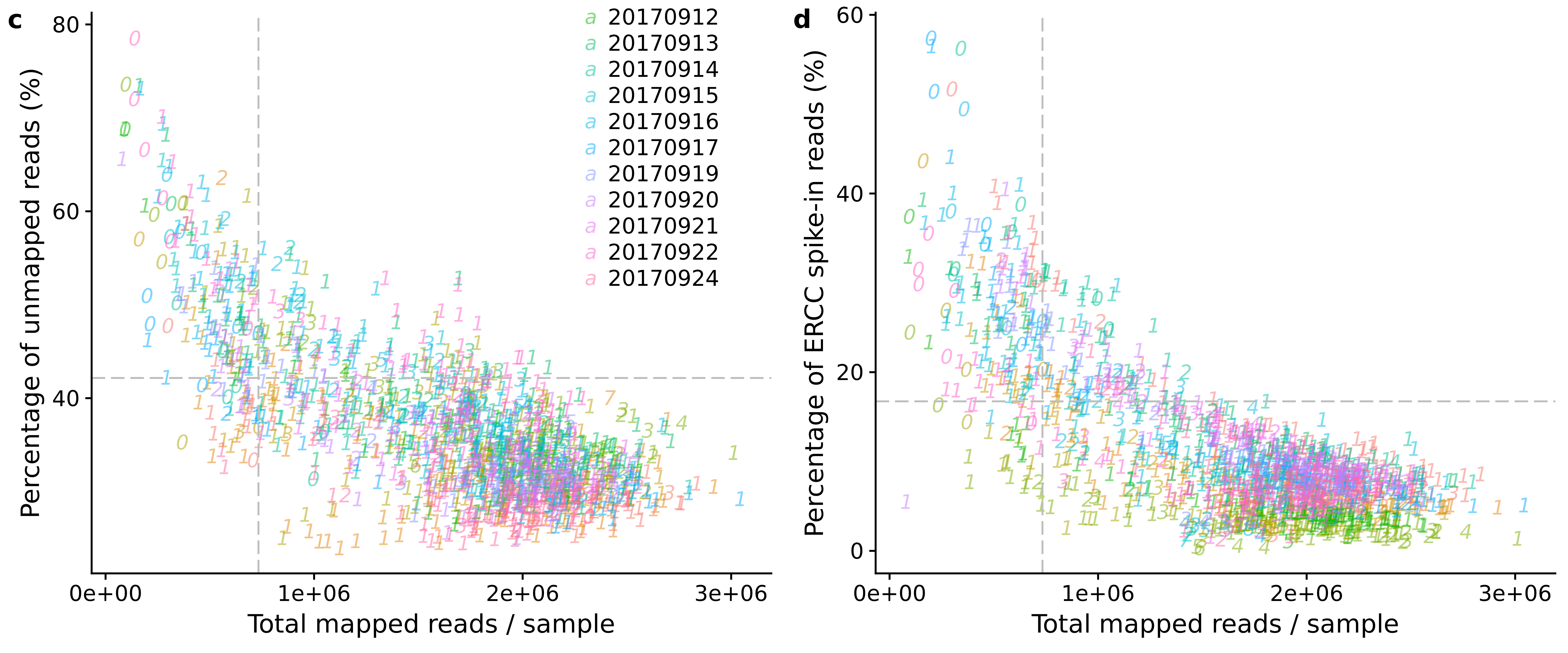
Output filters
\(~\)
These filters are later combined with metadata in our eset objects.
\(~\)
exps <- unique(anno$experiment)
for (index in 1:length(exps)) {
  tmp <- subset(anno,
                experiment == exps[index],
                select=c(cut_off_reads, unmapped_ratios, cut_off_unmapped,
                         ercc_percentage, cut_off_ercc, cut_off_genes,
                         ercc_conversion, conversion,
                         conversion_outlier, filter_all))
  tmp <- data.frame(sample_id=rownames(tmp), tmp)
  write.table(tmp,
              file = paste0("output/sampleqc.Rmd/",exps[index],".txt"),
              sep = "\t", quote = FALSE, col.names = TRUE, row.names = F)
}

# to import each text
#library(data.table)
#b <- fread("output/sampleqc.Rmd/20170905.txt", header=T)

pheno_labels <- rbind (
  c("cut_off_reads",
    "QC filter: number of mapped reads > 85th percentile among zero-cell samples"),
  c("unmapped_ratios",
    "QC filter: among reads with a valid UMI, number of unmapped/number of mapped (unmapped/umi)"),
  c("cut_off_unmapped",
    "QC filter: unmapped ratio < 30th percentile among zero-cell samples"),
  c("ercc_percentage",
    "QC filter: number of reads mapped to ERCC/total sample mapped reads (reads_ercc/mapped)"),
  c("cut_off_ercc",
    "QC filter: ercc percentage < 15th percentile among zero-cell samples"),
  c("cut_off_genes",
    "QC filter: number of endogeneous genes with at least one molecule (detect_hs) > 85th percentile among zero-cell samples"),
  c("ercc_conversion",
    "QC filter: among ERCC, number of molecules/number of mapped reads (mol_ercc/reads_ercc)"),
  c("conversion",
    "QC filter: among endogeneous genes, number of molecules/number of mapped reads (mol_hs/reads_hs)"),
  c("conversion_outlier",
    "QC filter: microscoy detects 1 cell AND ERCC conversion rate > .094"),
  c("filter_all",
    "QC filter: Does the sample pass all the QC filters? cell_number==1, mol_egfp >0, valid_id==1, cut_off_reads==TRUE, cut_off_ercc==TRUE, cut_off_genes=TRUE"))

write.table(pheno_labels,
            file = paste0("../output/sampleqc.Rmd/pheno_labels.txt"),
            sep = "\t", quote = FALSE, col.names = F, row.names = F)

#b <- fread("../output/sampleqc.Rmd/pheno_labels.txt", header=F)
Session information
R version 3.4.1 (2017-06-30)
Platform: x86_64-pc-linux-gnu (64-bit)
Running under: Scientific Linux 7.2 (Nitrogen)

Matrix products: default
BLAS: /project2/gilad/jdblischak/miniconda3/envs/fucci-seq/lib/R/lib/libRblas.so
LAPACK: /project2/gilad/jdblischak/miniconda3/envs/fucci-seq/lib/R/lib/libRlapack.so

locale:
 [1] LC_CTYPE=en_US.UTF-8       LC_NUMERIC=C
 [3] LC_TIME=en_US.UTF-8        LC_COLLATE=en_US.UTF-8
 [5] LC_MONETARY=en_US.UTF-8    LC_MESSAGES=en_US.UTF-8
 [7] LC_PAPER=en_US.UTF-8       LC_NAME=C
 [9] LC_ADDRESS=C               LC_TELEPHONE=C
[11] LC_MEASUREMENT=en_US.UTF-8 LC_IDENTIFICATION=C

attached base packages:
[1] parallel  methods   stats     graphics  grDevices utils     datasets
[8] base

other attached packages:
 [1] testit_0.6          MASS_7.3-45         Biobase_2.38.0
 [4] BiocGenerics_0.24.0 reshape2_1.4.2      edgeR_3.20.7
 [7] limma_3.34.6        dplyr_0.7.4         cowplot_0.9.1
[10] ggplot2_2.2.1

loaded via a namespace (and not attached):
 [1] Rcpp_0.12.13       RColorBrewer_1.1-2 compiler_3.4.1
 [4] git2r_0.19.0       plyr_1.8.4         bindr_0.1
 [7] tools_3.4.1        digest_0.6.12      evaluate_0.10.1
[10] tibble_1.3.3       gtable_0.2.0       lattice_0.20-34
[13] pkgconfig_2.0.1    rlang_0.1.2        yaml_2.1.14
[16] bindrcpp_0.2       stringr_1.2.0      knitr_1.16
[19] locfit_1.5-9.1     rprojroot_1.2      grid_3.4.1
[22] glue_1.1.1         R6_2.2.0           rmarkdown_1.6
[25] magrittr_1.5       backports_1.0.5    scales_0.5.0
[28] htmltools_0.3.6    assertthat_0.1     colorspace_1.3-2
[31] labeling_0.3       stringi_1.1.2      lazyeval_0.2.0
[34] munsell_0.4.3
This R Markdown site was created with workflowr