<!DOCTYPE html>

<html xmlns="http://www.w3.org/1999/xhtml">

<head>

<meta charset="utf-8" />
<meta http-equiv="Content-Type" content="text/html; charset=utf-8" />
<meta name="generator" content="pandoc" />


<meta name="author" content="Donghyung Lee" />

<meta name="date" content="2018-08-03" />

<title>scRNA-seq data simulation</title>

<script src="site_libs/jquery-1.11.3/jquery.min.js"></script>
<meta name="viewport" content="width=device-width, initial-scale=1" />
<link href="site_libs/bootstrap-3.3.5/css/united.min.css" rel="stylesheet" />
<script src="site_libs/bootstrap-3.3.5/js/bootstrap.min.js"></script>
<script src="site_libs/bootstrap-3.3.5/shim/html5shiv.min.js"></script>
<script src="site_libs/bootstrap-3.3.5/shim/respond.min.js"></script>
<script src="site_libs/navigation-1.1/tabsets.js"></script>
<link href="site_libs/highlightjs-9.12.0/textmate.css" rel="stylesheet" />
<script src="site_libs/highlightjs-9.12.0/highlight.js"></script>

<style type="text/css">code{white-space: pre;}</style>
<style type="text/css">
  pre:not([class]) {
    background-color: white;
  }
</style>
<script type="text/javascript">
if (window.hljs) {
  hljs.configure({languages: []});
  hljs.initHighlightingOnLoad();
  if (document.readyState && document.readyState === "complete") {
    window.setTimeout(function() { hljs.initHighlighting(); }, 0);
  }
}
</script>


<style type="text/css">
h1 {
  font-size: 34px;
}
h1.title {
  font-size: 38px;
}
h2 {
  font-size: 30px;
}
h3 {
  font-size: 24px;
}
h4 {
  font-size: 18px;
}
h5 {
  font-size: 16px;
}
h6 {
  font-size: 12px;
}
.table th:not([align]) {
  text-align: left;
}
</style>


</head>

<body>

<style type = "text/css">
.main-container {
  max-width: 940px;
  margin-left: auto;
  margin-right: auto;
}
code {
  color: inherit;
  background-color: rgba(0, 0, 0, 0.04);
}
img {
  max-width:100%;
  height: auto;
}
.tabbed-pane {
  padding-top: 12px;
}
button.code-folding-btn:focus {
  outline: none;
}
</style>


<style type="text/css">
/* padding for bootstrap navbar */
body {
  padding-top: 51px;
  padding-bottom: 40px;
}
/* offset scroll position for anchor links (for fixed navbar)  */
.section h1 {
  padding-top: 56px;
  margin-top: -56px;
}

.section h2 {
  padding-top: 56px;
  margin-top: -56px;
}
.section h3 {
  padding-top: 56px;
  margin-top: -56px;
}
.section h4 {
  padding-top: 56px;
  margin-top: -56px;
}
.section h5 {
  padding-top: 56px;
  margin-top: -56px;
}
.section h6 {
  padding-top: 56px;
  margin-top: -56px;
}
</style>

<script>
// manage active state of menu based on current page
$(document).ready(function () {
  // active menu anchor
  href = window.location.pathname
  href = href.substr(href.lastIndexOf('/') + 1)
  if (href === "")
    href = "index.html";
  var menuAnchor = $('a[href="' + href + '"]');

  // mark it active
  menuAnchor.parent().addClass('active');

  // if it's got a parent navbar menu mark it active as well
  menuAnchor.closest('li.dropdown').addClass('active');
});
</script>


<div class="container-fluid main-container">

<!-- tabsets -->
<script>
$(document).ready(function () {
  window.buildTabsets("TOC");
});
</script>

<!-- code folding -->


<div class="navbar navbar-default  navbar-fixed-top" role="navigation">
  <div class="container">
    <div class="navbar-header">
      <button type="button" class="navbar-toggle collapsed" data-toggle="collapse" data-target="#navbar">
        <span class="icon-bar"></span>
        <span class="icon-bar"></span>
        <span class="icon-bar"></span>
      </button>
      <a class="navbar-brand" href="index.html">iasvaExamples</a>
    </div>
    <div id="navbar" class="navbar-collapse collapse">
      <ul class="nav navbar-nav">
        <li>
  <a href="index.html">Home</a>
</li>
<li>
  <a href="license.html">License</a>
</li>
<li>
  <a href="https://github.com/dleelab/iasvaExamples">GitHub</a>
</li>
      </ul>
      <ul class="nav navbar-nav navbar-right">
        
      </ul>
    </div><!--/.nav-collapse -->
  </div><!--/.container -->
</div><!--/.navbar -->

<!-- Add a small amount of space between sections. -->
<style type="text/css">
div.section {
  padding-top: 12px;
}
</style>

<div class="fluid-row" id="header">


<h1 class="title toc-ignore">scRNA-seq data simulation</h1>
<h4 class="author"><em>Donghyung Lee</em></h4>
<h4 class="date"><em>2018-08-03</em></h4>

</div>

<div id="TOC">
<ul>
<li><a href="#load-packages">Load packages</a></li>
<li><a href="#load-the-islet-single-cell-rna-seq-data-n638-cells-and-26k-genes">Load the islet single cell RNA-Seq data (n=638 cells, and 26K genes)</a></li>
<li><a href="#look-at-mean-variance-relationship">Look at mean variance relationship</a></li>
<li><a href="#estimate-hidden-factors-using-usva-ssva-and-ia-sva-and-compare-them">Estimate hidden factors using USVA, SSVA and IA-SVA and compare them</a></li>
<li><a href="#session-information">Session information</a></li>
</ul>
</div>

<p><strong>Last updated:</strong> 2018-08-03</p>
<strong>workflowr checks:</strong> <small>(Click a bullet for more information)</small>
<ul>
<li>
<p><details> <summary> <strong style="color:blue;">✔</strong> <strong>R Markdown file:</strong> up-to-date </summary></p>
<p>Great! Since the R Markdown file has been committed to the Git repository, you know the exact version of the code that produced these results.</p>
</details>
</li>
<li>
<p><details> <summary> <strong style="color:blue;">✔</strong> <strong>Environment:</strong> empty </summary></p>
<p>Great job! The global environment was empty. Objects defined in the global environment can affect the analysis in your R Markdown file in unknown ways. For reproduciblity it’s best to always run the code in an empty environment.</p>
</details>
</li>
<li>
<p><details> <summary> <strong style="color:blue;">✔</strong> <strong>Seed:</strong> <code>set.seed(20180731)</code> </summary></p>
<p>The command <code>set.seed(20180731)</code> was run prior to running the code in the R Markdown file. Setting a seed ensures that any results that rely on randomness, e.g. subsampling or permutations, are reproducible.</p>
</details>
</li>
<li>
<p><details> <summary> <strong style="color:blue;">✔</strong> <strong>Session information:</strong> recorded </summary></p>
<p>Great job! Recording the operating system, R version, and package versions is critical for reproducibility.</p>
</details>
</li>
<li>
<p><details> <summary> <strong style="color:blue;">✔</strong> <strong>Repository version:</strong> <a href="https://github.com/dleelab/iasvaExamples/tree/18ea3c66646b609e44e9c33f0be38ba43a14f05e" target="_blank">18ea3c6</a> </summary></p>
Great! You are using Git for version control. Tracking code development and connecting the code version to the results is critical for reproducibility. The version displayed above was the version of the Git repository at the time these results were generated. <br><br> Note that you need to be careful to ensure that all relevant files for the analysis have been committed to Git prior to generating the results (you can use <code>wflow_publish</code> or <code>wflow_git_commit</code>). workflowr only checks the R Markdown file, but you know if there are other scripts or data files that it depends on. Below is the status of the Git repository when the results were generated:
<pre><code>
Ignored files:
    Ignored:    .DS_Store
    Ignored:    .Rhistory
    Ignored:    .Rproj.user/
    Ignored:    data/.DS_Store
    Ignored:    inst/.DS_Store
    Ignored:    inst/doc/.DS_Store
    Ignored:    vignettes/.DS_Store

Untracked files:
    Untracked:  Clustering_analyses_figure4_islets_sv1_3.pdf
    Untracked:  analysis/figure/
    Untracked:  docs/figure/Brain_scRNASeq_neuron_vs_oligodendrocyte_single_run.Rmd/
    Untracked:  docs/figure/hidden_heterogeneity_glioblastoma.Rmd/
    Untracked:  docs/figure/tSNE_post_IA-SVA_3celltypes.Rmd/
    Untracked:  docs/figure/tSNE_post_IA-SVA_Xin_Islets.Rmd/
    Untracked:  output/Brain_scRNASeq_neuron_astro_190_cells.pdf
    Untracked:  output/Brain_scRNASeq_neuron_astro_190_cells_run_time.pdf
    Untracked:  output/CC_genes.long.txt
    Untracked:  output/CC_genes.short.txt
    Untracked:  output/Clustering_analyses_figure3_sv1.pdf
    Untracked:  output/Clustering_analyses_figure4_Xin.pdf
    Untracked:  output/Clustering_analyses_figure4_Xin_sv1.pdf
    Untracked:  output/FigureS11_Xin_Islets_AllCells_IASVA_Markers_pheatmap.pdf
    Untracked:  output/Lawlor_Islets_3Cells_CellView_Seurat_FigS.pdf
    Untracked:  output/Lawlor_Islets_3Cells_IASVA_SV1SV3_rsqcutoff0.3_pheatmap_iasvaV0.95_Figure4_C.pdf
    Untracked:  output/Lawlor_Islets_3Cells_IASVA_SV4_rsqcutoff0.3_pheatmap_iasvaV0.95.pdf
    Untracked:  output/Lawlor_Islets_3Cells_IASVA_pairs4SVs_iasvaV0.95_black_FigS6.pdf
    Untracked:  output/Lawlor_Islets_3Cells_IASVA_pairs4SVs_iasvaV0.95_color_FigS6.pdf
    Untracked:  output/Lawlor_Islets_3Cells_SV1_SV3_Cell_Type_Genes_rsqcutoff0.3.txt
    Untracked:  output/Lawlor_Islets_3Cells_SV4_Genes_rsqcutoff0.3.txt
    Untracked:  output/Lawlor_Islets_3Cells_tSNE_IA-SVA_Fig4AB.pdf
    Untracked:  output/Patel_Glioblastoma_MGH30_CellCycle_Figure3ABCD.pdf
    Untracked:  output/Patel_Glioblastoma_MGH30_Cellcycle_SV1_Genes_rsqcutoff0.3.txt
    Untracked:  output/Patel_Glioblastoma_MGH30_Cellcycle_SV1_Genes_rsqcutoff0.4.txt
    Untracked:  output/Patel_Glioblastoma_MGH30_iasva_SV1_genes_rsqcutoff0.3_pheatmap_iasvaV0.95_Figure3F.pdf
    Untracked:  output/Xin_Islets_AllCells_IASVA.pdf
    Untracked:  output/Xin_Islets_AllCells_IASVA_nocolor.pdf
    Untracked:  output/Xin_Islets_AllCells_PCA.pdf
    Untracked:  output/Xin_Islets_AllCells_SV1_Genes_rsqcutoff0.2.txt
    Untracked:  output/Xin_Islets_AllCells_SV1_Genes_rsqcutoff0.3.txt
    Untracked:  output/Xin_Islets_AllCells_SV3_Genes_rsqcutoff0.2.txt
    Untracked:  output/Xin_Islets_AllCells_SV3_Genes_rsqcutoff0.3.txt
    Untracked:  output/Xin_Islets_AllCells_USVA.pdf
    Untracked:  output/Xin_Islets_AllCells_tSNEByKnownFactors_FigureS9.pdf
    Untracked:  output/Xin_Islets_All_demensionality_reduction_Figure4DEFG.pdf

</code></pre>
Note that any generated files, e.g. HTML, png, CSS, etc., are not included in this status report because it is ok for generated content to have uncommitted changes. </details>
</li>
</ul>
<details> <summary> <small><strong>Expand here to see past versions:</strong></small> </summary>
<ul>
<table style="border-collapse:separate; border-spacing:5px;">
<thead>
<tr>
<th style="text-align:left;">
File
</th>
<th style="text-align:left;">
Version
</th>
<th style="text-align:left;">
Author
</th>
<th style="text-align:left;">
Date
</th>
<th style="text-align:left;">
Message
</th>
</tr>
</thead>
<tbody>
<tr>
<td style="text-align:left;">
Rmd
</td>
<td style="text-align:left;">
<a href="https://github.com/dleelab/iasvaExamples/blob/18ea3c66646b609e44e9c33f0be38ba43a14f05e/analysis/scRNASeq_simulation.Rmd" target="_blank">18ea3c6</a>
</td>
<td style="text-align:left;">
dleelab
</td>
<td style="text-align:left;">
2018-08-03
</td>
<td style="text-align:left;">
error corrected
</td>
</tr>
<tr>
<td style="text-align:left;">
Rmd
</td>
<td style="text-align:left;">
<a href="https://github.com/dleelab/iasvaExamples/blob/c241b04dac899407045051a04b7539237f4d183f/analysis/scRNASeq_simulation.Rmd" target="_blank">c241b04</a>
</td>
<td style="text-align:left;">
dleelab
</td>
<td style="text-align:left;">
2018-08-03
</td>
<td style="text-align:left;">
added
</td>
</tr>
</tbody>
</table>
</ul>
<p></details></p>
<hr />
<p>To make simulation studies more objective, we used a simulation design suggested by the author of svaseq (<a href="http://jtleek.com/svaseq/simulateData.html" class="uri">http://jtleek.com/svaseq/simulateData.html</a>). We slightly modified the original design to simulate realistic single cell RNA sequencing (scRNA-seq) data sets (read counts with a high dropout rate) and multiple correlated hidden factors. We simulated baseline scRNA-seq data using the Polyester R package (<a href="https://bioconductor.org/packages/release/bioc/html/polyester.html" class="uri">https://bioconductor.org/packages/release/bioc/html/polyester.html</a>) by using the zero-inflated negative binomial distribution parameters estimated from a real-world scRNA-seq data obtained from human pancreatic islet samples (<a href="http://genome.cshlp.org/content/early/2017/01/16/gr.212720.116">Lawlor et. al., 2016</a>). The islet scRNA-seq dataset is included in a R data package (“iasvaExamples”) containing data examples for IA-SVA (<a href="https://github.com/dleelab/iasvaExamples" class="uri">https://github.com/dleelab/iasvaExamples</a>). To install the ‘iasvaExamples’ package, follow the instruction provided in the GitHub page.</p>
<div id="load-packages" class="section level2">
<h2>Load packages</h2>
<pre class="r"><code>rm(list=ls())
library(iasva)
library(iasvaExamples)
library(polyester)
library(sva)
library(corrplot)
library(DescTools) #pcc i.e., Pearson&#39;s contingency coefficient
library(RColorBrewer)
library(SummarizedExperiment)
color.vec &lt;- brewer.pal(8, &quot;Set1&quot;)</code></pre>
</div>
<div id="load-the-islet-single-cell-rna-seq-data-n638-cells-and-26k-genes" class="section level2">
<h2>Load the islet single cell RNA-Seq data (n=638 cells, and 26K genes)</h2>
<pre class="r"><code>data(&quot;Lawlor_Islet_scRNAseq_Read_Counts&quot;)
data(&quot;Lawlor_Islet_scRNAseq_Annotations&quot;)
ls()</code></pre>
<pre><code>[1] &quot;color.vec&quot;                         &quot;Lawlor_Islet_scRNAseq_Annotations&quot;
[3] &quot;Lawlor_Islet_scRNAseq_Read_Counts&quot;</code></pre>
<pre class="r"><code>counts &lt;- Lawlor_Islet_scRNAseq_Read_Counts
anns &lt;- Lawlor_Islet_scRNAseq_Annotations
dim(anns)</code></pre>
<pre><code>[1] 638  26</code></pre>
<pre class="r"><code>dim(counts)</code></pre>
<pre><code>[1] 26542   638</code></pre>
<pre class="r"><code>summary(anns)</code></pre>
<pre><code>     run             cell.type             COL1A1          INS       
 Length:638         Length:638         Min.   :1.00   Min.   :1.000  
 Class :character   Class :character   1st Qu.:1.00   1st Qu.:1.000  
 Mode  :character   Mode  :character   Median :1.00   Median :1.000  
                                       Mean   :1.03   Mean   :1.414  
                                       3rd Qu.:1.00   3rd Qu.:2.000  
                                       Max.   :2.00   Max.   :2.000  
                                                                     
     PRSS1            SST             GCG            KRT19      
 Min.   :1.000   Min.   :1.000   Min.   :1.000   Min.   :1.000  
 1st Qu.:1.000   1st Qu.:1.000   1st Qu.:1.000   1st Qu.:1.000  
 Median :1.000   Median :1.000   Median :1.000   Median :1.000  
 Mean   :1.038   Mean   :1.039   Mean   :1.375   Mean   :1.044  
 3rd Qu.:1.000   3rd Qu.:1.000   3rd Qu.:2.000   3rd Qu.:1.000  
 Max.   :2.000   Max.   :2.000   Max.   :2.000   Max.   :2.000  
                                                                
      PPY          num.genes             Cell_ID        UNOS_ID   
 Min.   :1.000   Min.   :3529   10th_C1_S59  :  1   ACCG268 :136  
 1st Qu.:1.000   1st Qu.:5270   10th_C10_S104:  1   ACJV399 :108  
 Median :1.000   Median :6009   10th_C11_S96 :  1   ACEL337 :103  
 Mean   :1.028   Mean   :5981   10th_C13_S61 :  1   ACIW009 : 93  
 3rd Qu.:1.000   3rd Qu.:6676   10th_C14_S53 :  1   ACCR015A: 57  
 Max.   :2.000   Max.   :8451   10th_C16_S105:  1   ACIB065 : 57  
                                (Other)      :632   (Other) : 84  
      Age        Biomaterial_Provider    Gender              Phenotype  
 Min.   :22.00   IIDP      : 45       Female:303   Non-Diabetic   :380  
 1st Qu.:29.00   Prodo Labs:593       Male  :335   Type 2 Diabetic:258  
 Median :42.00                                                          
 Mean   :39.63                                                          
 3rd Qu.:53.00                                                          
 Max.   :56.00                                                          
                                                                        
               Race          BMI          Cell_Type     Patient_ID 
 African American:175   Min.   :22.00   INS    :264   P1     :136  
 Hispanic        :165   1st Qu.:26.60   GCG    :239   P8     :108  
 White           :298   Median :32.95   KRT19  : 28   P3     :103  
                        Mean   :32.85   SST    : 25   P7     : 93  
                        3rd Qu.:35.80   PRSS1  : 24   P5     : 57  
                        Max.   :55.00   none   : 21   P6     : 57  
                                        (Other): 37   (Other): 84  
 Sequencing_Run Batch       Coverage       Percent_Aligned 
 12t    : 57    B1:193   Min.   :1206135   Min.   :0.8416  
 4th    : 57    B2:148   1st Qu.:2431604   1st Qu.:0.8769  
 9th    : 57    B3:297   Median :3042800   Median :0.8898  
 10t    : 56             Mean   :3160508   Mean   :0.8933  
 7th    : 55             3rd Qu.:3871697   3rd Qu.:0.9067  
 3rd    : 53             Max.   :5931638   Max.   :0.9604  
 (Other):303                                               
 Mitochondrial_Fraction Num_Expressed_Genes
 Min.   :0.003873       Min.   :3529       
 1st Qu.:0.050238       1st Qu.:5270       
 Median :0.091907       Median :6009       
 Mean   :0.108467       Mean   :5981       
 3rd Qu.:0.142791       3rd Qu.:6676       
 Max.   :0.722345       Max.   :8451       
                                           </code></pre>
<pre class="r"><code>ContCoef(table(anns$Gender, anns$Cell_Type))</code></pre>
<pre><code>[1] 0.225969</code></pre>
<pre class="r"><code>ContCoef(table(anns$Phenotype, anns$Cell_Type))</code></pre>
<pre><code>[1] 0.1145096</code></pre>
<pre class="r"><code>ContCoef(table(anns$Race, anns$Cell_Type))</code></pre>
<pre><code>[1] 0.3084146</code></pre>
<pre class="r"><code>ContCoef(table(anns$Patient_ID, anns$Cell_Type))</code></pre>
<pre><code>[1] 0.5232058</code></pre>
<pre class="r"><code>ContCoef(table(anns$Batch, anns$Cell_Type))</code></pre>
<pre><code>[1] 0.3295619</code></pre>
</div>
<div id="look-at-mean-variance-relationship" class="section level2">
<h2>Look at mean variance relationship</h2>
<pre class="r"><code>plot(rowMeans(log(counts+1)),rowVars(log(counts+1)),pch=19,col=color.vec[2])</code></pre>
<p><img src="figure/scRNASeq_simulation.Rmd/mean_var_relationship-1.png" width="672" style="display: block; margin: auto;" /></p>
<div id="estimate-zero-inflated-negative-binomial-parameters-from-the-islet-data" class="section level4">
<h4>
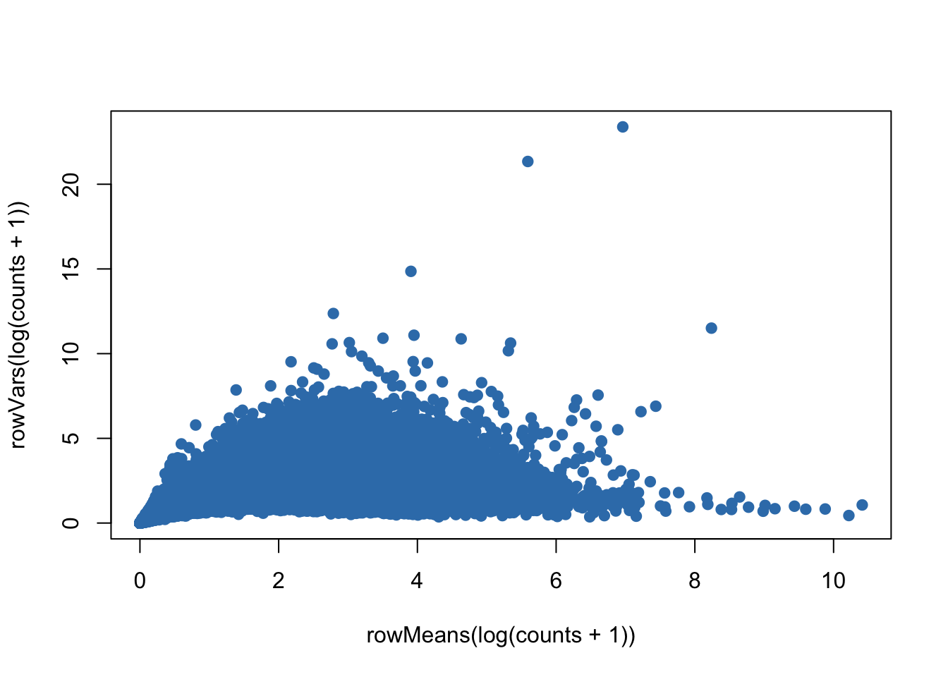
Estimate zero inflated negative binomial parameters from the islet data</h4>
<pre class="r"><code>## Estimate the zero inflated negative binomial parameters
#set.seed(12345)
set.seed(2018)
params = get_params(counts)</code></pre>
</div>
<div id="simulate-a-scrna-seq-data-set-affected-by-a-known-factor-and-three-hidden-factors" class="section level4">
<h4>Simulate a scRNA-seq data set affected by a known factor and three hidden factors</h4>
<pre class="r"><code>sample.size &lt;- 50
num.genes &lt;- 10000
prop.kfactor.genes &lt;- 0.1    #known factor
prop.hfactor1.genes &lt;- 0.3   #hidden factor1
prop.hfactor2.genes &lt;- 0.2   #hidden factor2
prop.hfactor3.genes &lt;- 0.1   #hidden factor3

num.kfactor.genes &lt;- num.genes*prop.kfactor.genes
num.hfactor1.genes &lt;- num.genes*prop.hfactor1.genes
num.hfactor2.genes &lt;- num.genes*prop.hfactor2.genes
num.hfactor3.genes &lt;- num.genes*prop.hfactor3.genes

factor.prop &lt;- 0.5
flip.prob &lt;- 0.8 # high corrleation between factors 
#flip.prob &lt;- 0.5 # row correlation between factors

# make first 10% of genes affected by the known factor.
kfactor = c(rep(-1,each=sample.size*factor.prop),rep(1,each=sample.size-(sample.size*factor.prop)))

coinflip = rbinom(sample.size,size=1,prob=flip.prob)
hfactor1 = kfactor*coinflip + -kfactor*(1-coinflip)
coinflip = rbinom(sample.size,size=1,prob=flip.prob)
hfactor2 = kfactor*coinflip + -kfactor*(1-coinflip)
coinflip = rbinom(sample.size,size=1,prob=flip.prob)
hfactor3 = kfactor*coinflip + -kfactor*(1-coinflip)

corrplot.mixed(cor(cbind(kfactor,hfactor1,hfactor2,hfactor3)))</code></pre>
<p><img src="figure/scRNASeq_simulation.Rmd/simulate_data-1.png" width="768" style="display: block; margin: auto;" /></p>
<pre class="r"><code>hfactor.mat &lt;- cbind(hfactor1,hfactor2,hfactor3)
kfcoeffs = c(rnorm(num.kfactor.genes),rep(0,num.genes-num.kfactor.genes))
nullindex= (num.kfactor.genes+1):num.genes

hfcoeffs1 &lt;- rep(0,num.genes)
hfcoeffs2 &lt;- rep(0,num.genes)
hfcoeffs3 &lt;- rep(0,num.genes)

## genes affected by each hidden factor is randomly selected.
hfcoeffs1[sample(1:num.genes, num.hfactor1.genes)] &lt;- rnorm(num.hfactor1.genes, sd=1)
hfcoeffs2[sample(1:num.genes, num.hfactor2.genes)] &lt;- rnorm(num.hfactor2.genes, sd=1)
hfcoeffs3[sample(1:num.genes, num.hfactor3.genes)] &lt;- rnorm(num.hfactor3.genes, sd=1)

coeffs = cbind(hfcoeffs1, hfcoeffs2, hfcoeffs3, kfcoeffs)
controls = ((hfcoeffs1!=0)|(hfcoeffs2!=0)|(hfcoeffs3!=0))&amp;(kfcoeffs==0)

par(mfrow=c(5,1))
plot(kfcoeffs)
plot(hfcoeffs1)
plot(hfcoeffs2)
plot(hfcoeffs3)
plot(controls)</code></pre>
<p><img src="figure/scRNASeq_simulation.Rmd/simulate_data-2.png" width="768" style="display: block; margin: auto;" /></p>
<pre class="r"><code>par(mfrow=c(1,1))

mod = model.matrix(~-1 + hfactor1 + hfactor2 + hfactor3 + kfactor)

dat0 = create_read_numbers(params$mu,params$fit,
                                     params$p0,beta=coeffs,mod=mod)

sum(dat0==0)/length(dat0)</code></pre>
<pre><code>[1] 0.681446</code></pre>
<pre class="r"><code>filter = apply(dat0, 1, function(x) length(x[x&gt;5])&gt;=3)
dat0 = dat0[filter,]
sum(dat0==0)/length(dat0)</code></pre>
<pre><code>[1] 0.52831</code></pre>
<pre class="r"><code>controls &lt;- controls[filter]

dim(dat0)</code></pre>
<pre><code>[1] 6580   50</code></pre>
<pre class="r"><code>dim(mod)</code></pre>
<pre><code>[1] 50  4</code></pre>
</div>
</div>
<div id="estimate-hidden-factors-using-usva-ssva-and-ia-sva-and-compare-them" class="section level2">
<h2>Estimate hidden factors using USVA, SSVA and IA-SVA and compare them</h2>
<pre class="r"><code>## set null and alternative models
mod1 = model.matrix(~kfactor)
mod0 = cbind(mod1[,1])

## Estimate hidden factors with unsuprvised SVA
usva.res = svaseq(dat0,mod1,mod0)$sv</code></pre>
<pre><code>Number of significant surrogate variables is:  3 
Iteration (out of 5 ):1  2  3  4  5  </code></pre>
<pre class="r"><code>cor(hfactor1, usva.res[,1])</code></pre>
<pre><code>[1] -0.9291762</code></pre>
<pre class="r"><code>cor(hfactor2, usva.res[,2])</code></pre>
<pre><code>[1] 0.6278626</code></pre>
<pre class="r"><code>cor(hfactor3, usva.res[,3])</code></pre>
<pre><code>[1] -0.5382027</code></pre>
<pre class="r"><code>## Estimate hidden factors with supervised SVA
ssva.res = svaseq(dat0,mod1,mod0,controls=controls)$sv</code></pre>
<pre><code>sva warning: controls provided so supervised sva is being performed.
Number of significant surrogate variables is:  3 </code></pre>
<pre class="r"><code>cor(hfactor1, ssva.res[,1])</code></pre>
<pre><code>[1] -0.9270694</code></pre>
<pre class="r"><code>cor(hfactor2, ssva.res[,2])</code></pre>
<pre><code>[1] -0.6297534</code></pre>
<pre class="r"><code>cor(hfactor3, ssva.res[,3])</code></pre>
<pre><code>[1] -0.5628941</code></pre>
<pre class="r"><code>## Estimate hidden factors with IA-SVA
summ_exp &lt;- SummarizedExperiment(assays = dat0)
iasva.res &lt;- iasva(summ_exp, as.matrix(mod1[,-1]), num.p = 20)$sv # the default number of permutations in SVA = 20</code></pre>
<pre><code>IA-SVA running...</code></pre>
<pre><code>
SV 1 Detected!</code></pre>
<pre><code>
SV 2 Detected!</code></pre>
<pre><code>
SV 3 Detected!</code></pre>
<pre><code>
# of significant surrogate variables: 3</code></pre>
<pre class="r"><code>cor(hfactor1, iasva.res[,1])</code></pre>
<pre><code>[1] -0.9944336</code></pre>
<pre class="r"><code>cor(hfactor2, iasva.res[,2])</code></pre>
<pre><code>[1] 0.9901559</code></pre>
<pre class="r"><code>cor(hfactor3, iasva.res[,3])</code></pre>
<pre><code>[1] 0.9797604</code></pre>
<pre class="r"><code>hf1.mat &lt;- cbind(hfactor1, usva.res[,1], ssva.res[,1], iasva.res[,1])
hf2.mat &lt;- cbind(hfactor2, usva.res[,2], ssva.res[,2], iasva.res[,2])
hf3.mat &lt;- cbind(hfactor3, usva.res[,3], ssva.res[,3], iasva.res[,3])
colnames(hf1.mat) &lt;- c(&quot;HF1&quot;, &quot;USVA&quot;, &quot;SSVA&quot;, &quot;IA-SVA&quot;)
colnames(hf2.mat) &lt;- c(&quot;HF2&quot;, &quot;USVA&quot;, &quot;SSVA&quot;, &quot;IA-SVA&quot;)
colnames(hf3.mat) &lt;- c(&quot;HF3&quot;, &quot;USVA&quot;, &quot;SSVA&quot;, &quot;IA-SVA&quot;)

par(mfrow=c(2,2))
corrplot.mixed(abs(cor(hf1.mat)), tl.pos=&quot;lt&quot;)
corrplot.mixed(abs(cor(hf2.mat)), tl.pos=&quot;lt&quot;)
corrplot.mixed(abs(cor(hf3.mat)), tl.pos=&quot;lt&quot;)</code></pre>
<p><img src="figure/scRNASeq_simulation.Rmd/hidden_factor_estimation-1.png" width="960" style="display: block; margin: auto;" /></p>
</div>
<div id="session-information" class="section level2">
<h2>Session information</h2>
<pre class="r"><code>sessionInfo()</code></pre>
<pre><code>R version 3.5.0 (2018-04-23)
Platform: x86_64-apple-darwin15.6.0 (64-bit)
Running under: macOS Sierra 10.12.6

Matrix products: default
BLAS: /Library/Frameworks/R.framework/Versions/3.5/Resources/lib/libRblas.0.dylib
LAPACK: /Library/Frameworks/R.framework/Versions/3.5/Resources/lib/libRlapack.dylib

locale:
[1] en_US.UTF-8/en_US.UTF-8/en_US.UTF-8/C/en_US.UTF-8/en_US.UTF-8

attached base packages:
[1] parallel  stats4    stats     graphics  grDevices utils     datasets 
[8] methods   base     

other attached packages:
 [1] SummarizedExperiment_1.10.1 DelayedArray_0.6.1         
 [3] matrixStats_0.53.1          Biobase_2.40.0             
 [5] GenomicRanges_1.32.3        GenomeInfoDb_1.16.0        
 [7] IRanges_2.14.10             S4Vectors_0.18.3           
 [9] BiocGenerics_0.26.0         RColorBrewer_1.1-2         
[11] DescTools_0.99.24           corrplot_0.84              
[13] sva_3.28.0                  BiocParallel_1.14.2        
[15] genefilter_1.62.0           mgcv_1.8-23                
[17] nlme_3.1-137                polyester_1.16.0           
[19] iasvaExamples_1.0.0         iasva_0.99.3               

loaded via a namespace (and not attached):
 [1] Rcpp_0.12.17           mvtnorm_1.0-8          lattice_0.20-35       
 [4] Biostrings_2.48.0      rprojroot_1.3-2        digest_0.6.15         
 [7] backports_1.1.2        RSQLite_2.1.1          evaluate_0.10.1       
[10] zlibbioc_1.26.0        annotate_1.58.0        irlba_2.3.2           
[13] whisker_0.3-2          blob_1.1.1             R.utils_2.6.0         
[16] R.oo_1.22.0            Matrix_1.2-14          rmarkdown_1.9         
[19] splines_3.5.0          stringr_1.3.1          foreign_0.8-70        
[22] RCurl_1.95-4.10        bit_1.1-14             compiler_3.5.0        
[25] manipulate_1.0.1       htmltools_0.3.6        expm_0.999-2          
[28] GenomeInfoDbData_1.1.0 workflowr_1.0.1        XML_3.98-1.11         
[31] MASS_7.3-50            bitops_1.0-6           R.methodsS3_1.7.1     
[34] grid_3.5.0             xtable_1.8-2           DBI_1.0.0             
[37] git2r_0.21.0           magrittr_1.5           stringi_1.2.2         
[40] XVector_0.20.0         limma_3.36.2           boot_1.3-20           
[43] tools_3.5.0            bit64_0.9-7            logspline_2.1.11      
[46] survival_2.42-3        yaml_2.1.19            AnnotationDbi_1.42.1  
[49] cluster_2.0.7-1        memoise_1.1.0          knitr_1.20            </code></pre>
</div>

<!-- Adjust MathJax settings so that all math formulae are shown using
TeX fonts only; see
http://docs.mathjax.org/en/latest/configuration.html.  This will make
the presentation more consistent at the cost of the webpage sometimes
taking slightly longer to load. Note that this only works because the
footer is added to webpages before the MathJax javascript. -->
<script type="text/x-mathjax-config">
  MathJax.Hub.Config({
    "HTML-CSS": { availableFonts: ["TeX"] }
  });
</script>

<hr>
<p>
  This reproducible <a href="http://rmarkdown.rstudio.com">R Markdown</a>
  analysis was created with
  <a href="https://github.com/jdblischak/workflowr">workflowr</a> 1.0.1
</p>
<hr>


</div>

<script>

// add bootstrap table styles to pandoc tables
function bootstrapStylePandocTables() {
  $('tr.header').parent('thead').parent('table').addClass('table table-condensed');
}
$(document).ready(function () {
  bootstrapStylePandocTables();
});


</script>

<!-- dynamically load mathjax for compatibility with self-contained -->
<script>
  (function () {
    var script = document.createElement("script");
    script.type = "text/javascript";
    script.src  = "https://mathjax.rstudio.com/latest/MathJax.js?config=TeX-AMS-MML_HTMLorMML";
    document.getElementsByTagName("head")[0].appendChild(script);
  })();
</script>

</body>
</html>