deNovo peak callling
Briana Mittleman
6/28/2018
Last updated: 2018-07-06
workflowr checks: (Click a bullet for more information)-
✔ R Markdown file: up-to-date
Great! Since the R Markdown file has been committed to the Git repository, you know the exact version of the code that produced these results.
-
✔ Environment: empty
Great job! The global environment was empty. Objects defined in the global environment can affect the analysis in your R Markdown file in unknown ways. For reproduciblity it’s best to always run the code in an empty environment.
-
✔ Seed:
set.seed(12345)The command
set.seed(12345)was run prior to running the code in the R Markdown file. Setting a seed ensures that any results that rely on randomness, e.g. subsampling or permutations, are reproducible. -
✔ Session information: recorded
Great job! Recording the operating system, R version, and package versions is critical for reproducibility.
-
Great! You are using Git for version control. Tracking code development and connecting the code version to the results is critical for reproducibility. The version displayed above was the version of the Git repository at the time these results were generated.✔ Repository version: 2522654
Note that you need to be careful to ensure that all relevant files for the analysis have been committed to Git prior to generating the results (you can usewflow_publishorwflow_git_commit). workflowr only checks the R Markdown file, but you know if there are other scripts or data files that it depends on. Below is the status of the Git repository when the results were generated:
Note that any generated files, e.g. HTML, png, CSS, etc., are not included in this status report because it is ok for generated content to have uncommitted changes.Ignored files: Ignored: .DS_Store Ignored: .Rhistory Ignored: .Rproj.user/ Ignored: output/.DS_Store Untracked files: Untracked: data/18486.genecov.txt Untracked: data/YL-SP-18486-T_S9_R1_001-genecov.txt Untracked: data/bedgraph_peaks/ Untracked: data/bin200.5.T.nuccov.bed Untracked: data/bin200.Anuccov.bed Untracked: data/bin200.nuccov.bed Untracked: data/gene_cov/ Untracked: data/leafcutter/ Untracked: data/nuc6up/ Untracked: data/reads_mapped_three_prime_seq.csv Untracked: data/ssFC200.cov.bed Untracked: output/picard/ Untracked: output/plots/ Untracked: output/qual.fig2.pdf Unstaged changes: Modified: analysis/dif.iso.usage.leafcutter.Rmd Modified: analysis/explore.filters.Rmd Modified: analysis/test.max2.Rmd Modified: code/Snakefile
Expand here to see past versions:
| File | Version | Author | Date | Message |
|---|---|---|---|---|
| Rmd | 2522654 | Briana Mittleman | 2018-07-06 | fix axis |
| html | a0541e3 | Briana Mittleman | 2018-07-06 | Build site. |
| Rmd | df5cfe4 | Briana Mittleman | 2018-07-06 | add Yangs peaks |
| html | 9de3677 | Briana Mittleman | 2018-07-05 | Build site. |
| Rmd | c619183 | Briana Mittleman | 2018-07-05 | examine long peaks |
| html | 2d67ec5 | Briana Mittleman | 2018-07-05 | Build site. |
| Rmd | 15c7967 | Briana Mittleman | 2018-07-05 | add split analysis |
| html | 24c6663 | Briana Mittleman | 2018-07-03 | Build site. |
| Rmd | 776fc62 | Briana Mittleman | 2018-07-03 | genome cov stats |
| html | b48f27c | Briana Mittleman | 2018-07-02 | Build site. |
| Rmd | 1e2ff4c | Briana Mittleman | 2018-07-02 | evaluate bedgraph regions |
Create Bedgraph
I will call peaks de novo in the combined total and nuclear fraction 3’ Seq. The data is reletevely clean so I will start with regions that have continuous coverage. I will first create a bedgraph.
#!/bin/bash

#SBATCH --job-name=Tbedgraph
#SBATCH --account=pi-yangili1
#SBATCH --time=24:00:00
#SBATCH --output=Tbedgraph.out
#SBATCH --error=Tbedgraph.err
#SBATCH --partition=broadwl
#SBATCH --mem=40G
#SBATCH --mail-type=END


module load Anaconda3
source activate three-prime-env

samtools sort -o /project2/gilad/briana/threeprimeseq/data/macs2/TotalBamFiles.sort.bam /project2/gilad/briana/threeprimeseq/data/macs2/TotalBamFiles.bam

bedtools genomecov -ibam /project2/gilad/briana/threeprimeseq/data/macs2/TotalBamFiles.sort.bam -bga > /project2/gilad/briana/threeprimeseq/data/bedgraph/TotalBamFiles.bedgraph
Next I will create the file without the 0 places in the genome. I will be able to use this for the bedtools merge function.
awk '{if ($4 != 0) print}' TotalBamFiles.bedgraph >TotalBamFiles_no0.bedgraph I can merge the regions with consequtive reads using the bedtools merge function.
-i input bed
-c colomn to act on
-o collapse, print deliminated list of the counts from -c call
-delim “,”
This is the mergeBedgraph.sh script. It takes in the no 0 begraph filename without the path.
#!/bin/bash

#SBATCH --job-name=merge
#SBATCH --account=pi-yangili1
#SBATCH --time=8:00:00
#SBATCH --output=merge.out
#SBATCH --error=merge.err
#SBATCH --partition=broadwl
#SBATCH --mem=16G
#SBATCH --mail-type=END

module load Anaconda3
source activate three-prime-env

bedgraph=$1
describer=$(echo ${bedgraph} | sed -e "s/.bedgraph$//")

bedtools merge -c 4,4,4 -o count,mean,collapse -delim "," -i /project2/gilad/briana/threeprimeseq/data/bedgraph/$1 > /project2/gilad/briana/threeprimeseq/data/bedgraph/${describer}.peaks.bed
Run this first on the total bedgraph, TotalBamFiles_no0.bedgraph. The file has chromosome, start, end, number of regions, mean, and a string of the values.
This is not exaclty what I want. I need to go back and do genome cov not collapsing with bedgraph.
To evaluate this I will bring the file into R and plot some statistics about it.
#!/bin/bash

#SBATCH --job-name=Tgencov
#SBATCH --account=pi-yangili1
#SBATCH --time=24:00:00
#SBATCH --output=Tgencov.out
#SBATCH --error=Tgencov.err
#SBATCH --partition=broadwl
#SBATCH --mem=40G
#SBATCH --mail-type=END


module load Anaconda3
source activate three-prime-env


bedtools genomecov -ibam /project2/gilad/briana/threeprimeseq/data/macs2/TotalBamFiles.sort.bam -d > /project2/gilad/briana/threeprimeseq/data/bedgraph/TotalBamFiles.genomecov.bed
I will now remove the bases with 0 coverage.
awk '{if ($3 != 0) print}' TotalBamFiles.genomecov.bed > TotalBamFiles.genomecov.no0.bed

awk '{print $1 "\t" $2 "\t"  $2 "\t" $3}' TotalBamFiles.genomecov.no0.bed > TotalBamFiles.genomecov.no0.fixed.bed
I will now merge the genomecov_no0 file with mergeGencov.sh
#!/bin/bash

#SBATCH --job-name=mergegc
#SBATCH --account=pi-yangili1
#SBATCH --time=8:00:00
#SBATCH --output=mergegc.out
#SBATCH --error=mergegc.err
#SBATCH --partition=broadwl
#SBATCH --mem=16G
#SBATCH --mail-type=END

module load Anaconda3
source activate three-prime-env

gencov=$1
describer=$(echo ${gencov} | sed -e "s/.genomecov.no0.fixed.bed$//")

bedtools merge -c 4,4,4 -o count,mean,collapse -delim "," -i /project2/gilad/briana/threeprimeseq/data/bedgraph/$1 > /project2/gilad/briana/threeprimeseq/data/bedgraph/${describer}.gencovpeaks.bed
This method gives us 811,637 regions.
Evaluate regions
Bedgraph results
library(dplyr)Warning: package 'dplyr' was built under R version 3.4.4
Attaching package: 'dplyr'The following objects are masked from 'package:stats':
filter, lagThe following objects are masked from 'package:base':
intersect, setdiff, setequal, unionlibrary(ggplot2)
library(readr)
library(workflowr)Loading required package: rmarkdownThis is workflowr version 1.0.1
Run ?workflowr for help getting startedlibrary(tidyr)First I will look at the bedgraph file. This is not as imformative becuase it combined regions with the same counts.
total_bedgraph=read.table("../data/bedgraph_peaks/TotalBamFiles_no0.peaks.bed",col.names = c("chr", "start", "end", "regions", "mean", "counts"))Plot the mean:
plot(sort(log10(total_bedgraph$mean), decreasing=T), xlab="Region", ylab="log10 of bedgraph region bin", main="Distribution of log10 region means from bedgraph")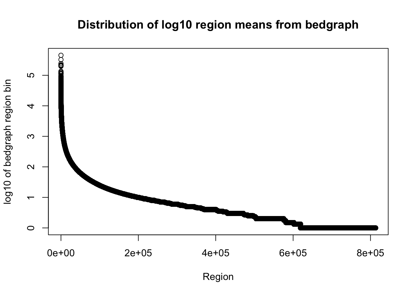
Expand here to see past versions of unnamed-chunk-9-1.png:
| Version | Author | Date |
|---|---|---|
| 24c6663 | Briana Mittleman | 2018-07-03 |
I want to look at the distribution of how many bases are included in the regions.
Tregion_bases=total_bedgraph %>% mutate(bases=end-start) %>% select(bases)Warning: package 'bindrcpp' was built under R version 3.4.4plot(sort(log10(Tregion_bases$bases), decreasing = T), xlab="Region", ylab="log10 of region size", main="Distribution of bases in regions- log10")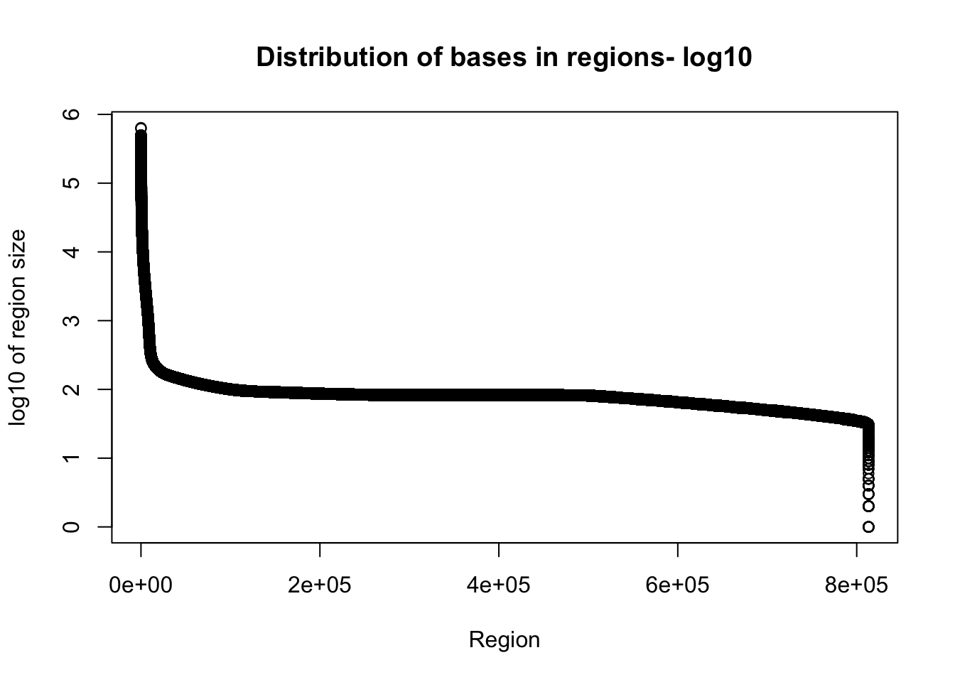
Expand here to see past versions of unnamed-chunk-10-1.png:
| Version | Author | Date |
|---|---|---|
| 24c6663 | Briana Mittleman | 2018-07-03 |
Given the reads are abotu 60bp this is probably pretty good.
GenomeCov results
I am only going to look at the number of bases in region and mean coverage columns here because the file is really big.
total_gencov=read.table("../data/bedgraph_peaks/TotalBamFiles.gencovpeaks_noregstring.bed",col.names = c("chr", "start", "end", "regions", "mean"))Plot the mean:
plot(sort(log10(total_gencov$mean), decreasing=T), xlab="Region", ylab="log10 of mean bin count", main="Distribution of log10 region means")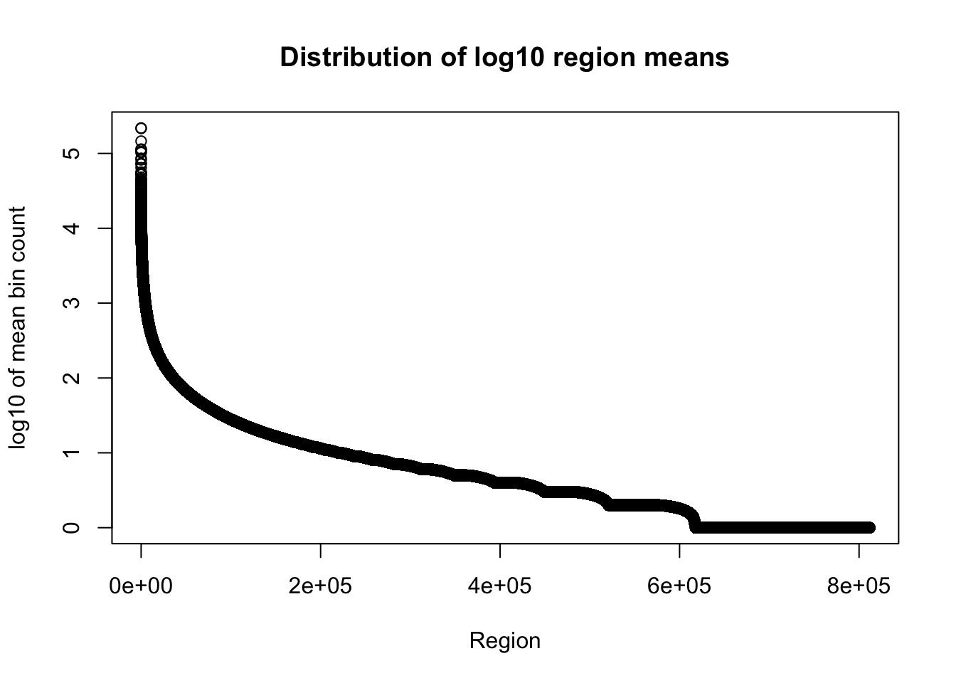
Expand here to see past versions of unnamed-chunk-12-1.png:
| Version | Author | Date |
|---|---|---|
| 24c6663 | Briana Mittleman | 2018-07-03 |
plot(sort(log10(total_gencov$regions), decreasing = T), xlab="Region", ylab="log10 of region size", main="Distribution of bases in regions- log10")
Expand here to see past versions of unnamed-chunk-13-1.png:
| Version | Author | Date |
|---|---|---|
| 24c6663 | Briana Mittleman | 2018-07-03 |
Plot number of bases against the mean:
ggplot(total_gencov, aes(y=log10(regions), x=log10(mean))) +
         geom_point(na.rm = TRUE, size = 0.1) +
         geom_density2d(na.rm = TRUE, size = 1, colour = 'red') +
         ylab('Log10 Region size') +
         xlab('Log10 Mean region coverage') +
        ggtitle("Region size vs Region Coverage: Combined Total Libraries")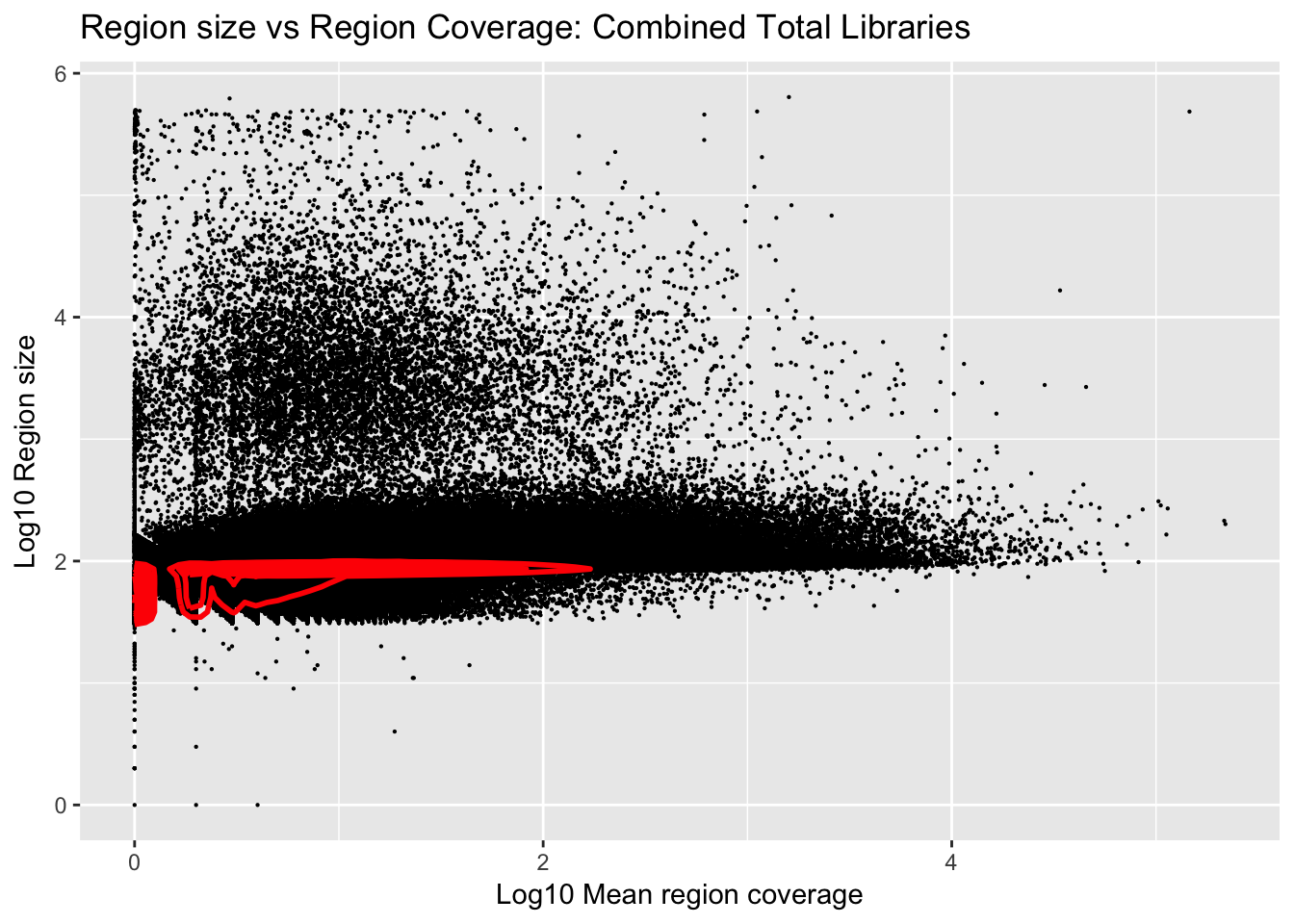
Expand here to see past versions of unnamed-chunk-14-1.png:
| Version | Author | Date |
|---|---|---|
| 24c6663 | Briana Mittleman | 2018-07-03 |
Troubleshooting
Account for split reads
In the previous analysis I did not account for split reads in the genome coveragre step. This may explain some of the long regions that are an effect of splicing. This script is
#!/bin/bash

#SBATCH --job-name=Tgencovsplit
#SBATCH --account=pi-yangili1
#SBATCH --time=24:00:00
#SBATCH --output=Tgencovsplit.out
#SBATCH --error=Tgencovaplit.err
#SBATCH --partition=broadwl
#SBATCH --mem=40G
#SBATCH --mail-type=END


module load Anaconda3
source activate three-prime-env


bedtools genomecov -ibam /project2/gilad/briana/threeprimeseq/data/macs2/TotalBamFiles.sort.bam -d -split > /project2/gilad/briana/threeprimeseq/data/bedgraph/TotalBamFiles.split.genomecov.bed
Now I need to remove the 0s and merge.
awk '{if ($3 != 0) print}' TotalBamFiles.split.genomecov.bed > TotalBamFiles.split.genomecov.no0.bed

awk '{print $1 "\t" $2 "\t"  $2 "\t" $3}' TotalBamFiles.split.genomecov.no0.bed > TotalBamFiles.split.genomecov.no0.fixed.bed
Use this file to run mergeGencov.sh.
total_gencov_split=read.table("../data/bedgraph_peaks/TotalBamFiles.split.gencovpeaks.noregstring.bed",col.names = c("chr", "start", "end", "regions", "mean"))Plot the region size. I expect some of the long regions are gone.
plot(sort(log10(total_gencov_split$regions), decreasing = T), xlab="Region", ylab="log10 of region size", main="Distribution of bases in regions- log10 SPLIT")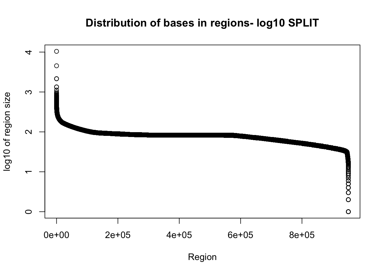
Expand here to see past versions of unnamed-chunk-18-1.png:
| Version | Author | Date |
|---|---|---|
| 2d67ec5 | Briana Mittleman | 2018-07-05 |
Plot the region size against the mean:
Plot number of bases against the mean:
splitplot=ggplot(total_gencov_split, aes(y=log10(regions), x=log10(mean))) +
         geom_point(na.rm = TRUE, size = 0.1) +
         geom_density2d(na.rm = TRUE, size = 1, colour = 'red') +
         ylab('Log10 Region size') +
         xlab('Log10 Mean region coverage') +
     scale_y_continuous(limits = c(0, 3)) +
        ggtitle("Combined Total Libraries SPLIT")
Investigate long regions
Some of the regions are long and probably represent 2 or more sites. This is evident in highly expressed genes such as actB. I will look at some of the long regions and make histograms with the strings of coverage in the region.
First I am going to look at chr11:65266512-65268654, this is peak 580475 I will go into the otalBamFiles.split.gencovpeaks.bed file and use:
grep -n 65266512 TotalBamFiles.split.gencovpeaks.bed | awk '{print $6}' > loc_ch11_65266512_65268654.txtloc_ch11_65266512_65268654=read.csv("../data/bedgraph_peaks/loc_ch11_65266512_65268654.txt", header=F) %>% t
loc_ch11_65266512_65268654_df= as.data.frame(loc_ch11_65266512_65268654)
loc_ch11_65266512_65268654_df$loc= seq(1:nrow(loc_ch11_65266512_65268654_df))
colnames(loc_ch11_65266512_65268654_df)= c("count", "loc")
ggplot(loc_ch11_65266512_65268654_df, aes(x=loc, y=count)) + geom_line() + labs(y="Read Count", x="Peak Location", title="Example of long region called as 1 peak \n ch11 65266512-65268654")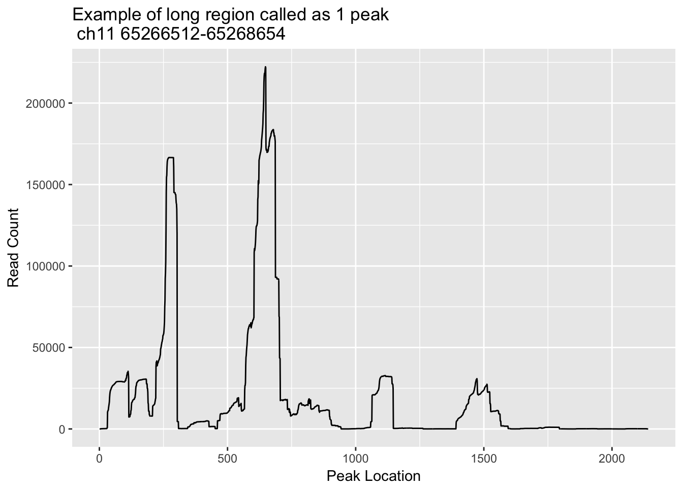
Expand here to see past versions of unnamed-chunk-21-1.png:
| Version | Author | Date |
|---|---|---|
| 9de3677 | Briana Mittleman | 2018-07-05 |
Try one more. Example. line 816811, chr:17- 79476983- 79477761
grep -n 79476983 TotalBamFiles.split.gencovpeaks.bed | awk '{print $6}' > loc_ch17_79476983_79477761.txtloc_ch17_79476983_79477761=read.csv("../data/bedgraph_peaks/loc_ch17_79476983_79477761.txt", header=F) %>% t
loc_ch17_79476983_79477761_df= as.data.frame(loc_ch17_79476983_79477761)
loc_ch17_79476983_79477761_df$loc= seq(1:nrow(loc_ch17_79476983_79477761_df))
colnames(loc_ch17_79476983_79477761_df)= c("count", "loc")
ggplot(loc_ch17_79476983_79477761_df, aes(x=loc, y=count)) + geom_line() + labs(y="Read Count", x="Peak Location", title="Example of long region called as 1 peak \n ch17 79476983:79477761")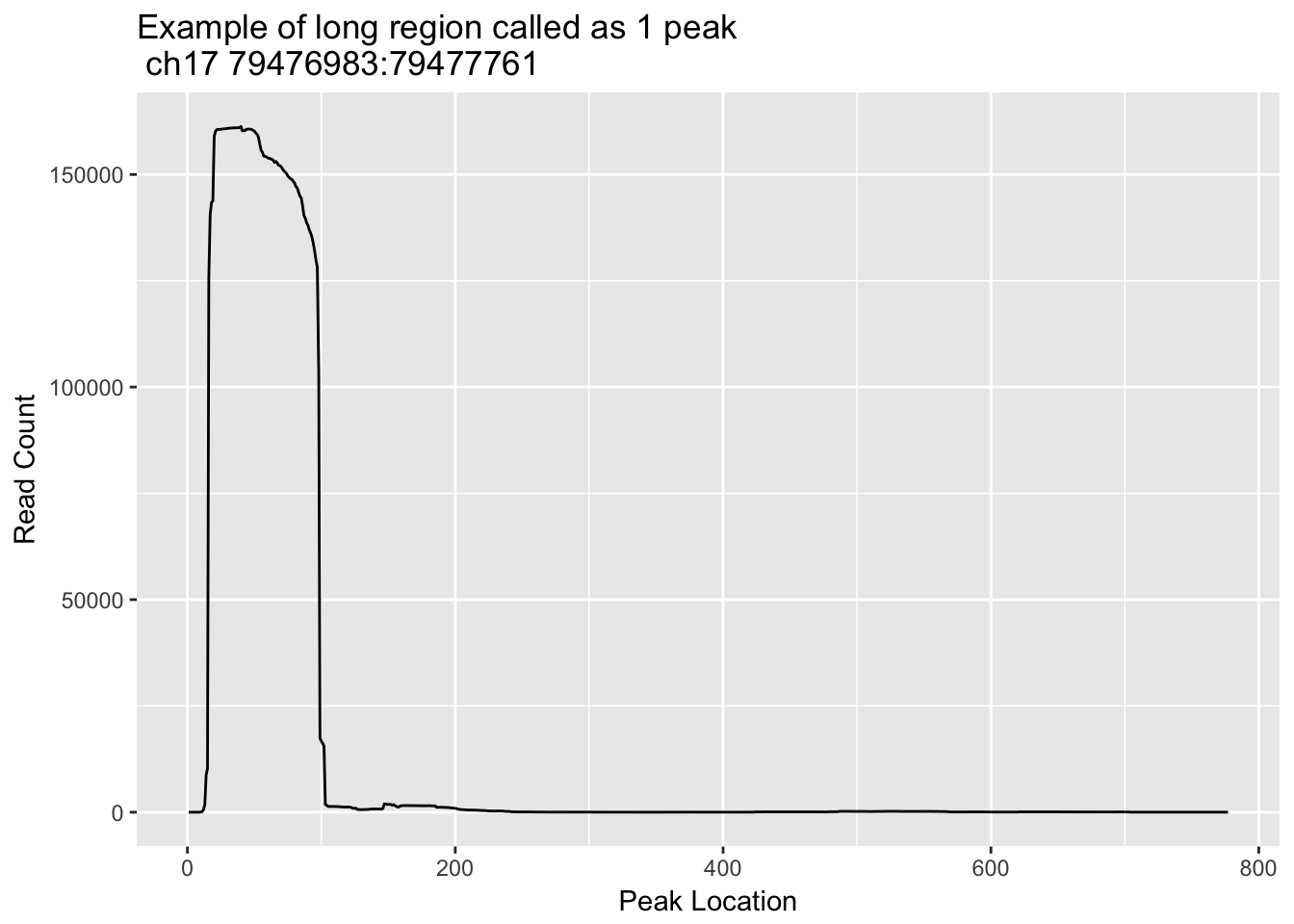
Expand here to see past versions of unnamed-chunk-23-1.png:
| Version | Author | Date |
|---|---|---|
| 9de3677 | Briana Mittleman | 2018-07-05 |
This one is not multiple peaks but it does need to be trimmed.
Yang created an adhoc method to do this.
def main(inFile, outFile, ctarget):
    fout = open(outFile,'w')
    mincount = 10
    ov = 20
    current_peak = []

    currentChrom = None

    for ln in open(inFile):
        chrom, pos, count = ln.split()
        if chrom != ctarget: continue
        count = float(count)
        if currentChrom == None:
            currentChrom = chrom

        if count == 0 or currentChrom != chrom:
            if len(current_peak) > 0:
                M = max([x[1] for x in current_peak])
                if M > mincount:
                    all_peaks = refine_peak(current_peak, M, M*0.1,M*0.05)
                    #refined_peaks = [(x[0][0],x[-1][0], np.mean([y[1] for y in x])) for x in all_peaks]
                    rpeaks = [(int(x[0][0])-ov,int(x[-1][0])+ov, np.mean([y[1] for y in x])) for x in all_peaks]
                    if len(rpeaks) > 1:
                        for clu in cluster_intervals(rpeaks)[0]:
                            M = max([x[2] for x in clu])
                            merging = []
                            for x in clu:
                                if x[2] > M *0.5:
                                    #print x, M
                                    merging.append(x)
                            c, s,e,mean =  chrom, min([x[0] for x in merging])+ov, max([x[1] for x in merging])-ov, np.mean([x[2] for x in merging])
                            #print c,s,e,mean
                            fout.write("chr%s\t%d\t%d\t%d\t+\t.\n"%(c,s,e,mean))
                            fout.flush()
                    elif len(rpeaks) == 1:
                        s,e,mean = rpeaks[0]
                        fout.write("chr%s\t%d\t%d\t%f\t+\t.\n"%(chrom,s+ov,e-ov,mean))
                        print "chr%s"%chrom+"\t%d\t%d\t%f\t+\t.\n"%rpeaks[0]
                    #print refined_peaks
            current_peak = []
        else:
            current_peak.append((pos,count))
        currentChrom = chrom
def refine_peak(current_peak, M, thresh, noise, minpeaksize=30):

    cpeak = []
    opeak = []
    allcpeaks = []
    allopeaks = []
    for pos, count in current_peak:
        if count > thresh:
            cpeak.append((pos,count))
            opeak = []
            continue
        elif count > noise:
            opeak.append((pos,count))
        else:
            if len(opeak) > minpeaksize:
                allopeaks.append(opeak)
            opeak = []
        if len(cpeak) > minpeaksize:
            allcpeaks.append(cpeak)
            cpeak = []

    if len(cpeak) > minpeaksize:
        allcpeaks.append(cpeak)
    if len(opeak) > minpeaksize:
        allopeaks.append(opeak)
    allpeaks = allcpeaks
    for opeak in allopeaks:
        M = max([x[1] for x in opeak])
        allpeaks += refine_peak(opeak, M, M*0.3, noise)
    #print [(x[0],x[-1]) for x in allcpeaks], [(x[0],x[-1]) for x in allopeaks], [(x[0],x[-1]) for x in allpeaks]
    #print '---\n'
    return allpeaks
if __name__ == "__main__":
    import numpy as np
    from misc_helper import *
    import sys
    chrom = sys.argv[1]
    inFile = "/project2/yangili1/threeprimeseq/gencov/TotalBamFiles.split.genomecov.bed"
    outFile = "APApeaks_chr%s.bed"%chrom
    main(inFile, outFile, chrom)
This is done by chromosome and takes in the TotalBam Split genome coverage file I made.I am going to look at the stats for these peaks.
YL_peaks=read.table("../data/bedgraph_peaks/APApeaks.bed", col.names = c("chr", "start", "end", "count", "strand", "score")) %>% mutate(length=end-start)Plot the lengths
plot(sort(log10(YL_peaks$length), decreasing = T), xlab="Region", ylab="log10 of region size", main="Distribution of bases in YL regions- log10 ")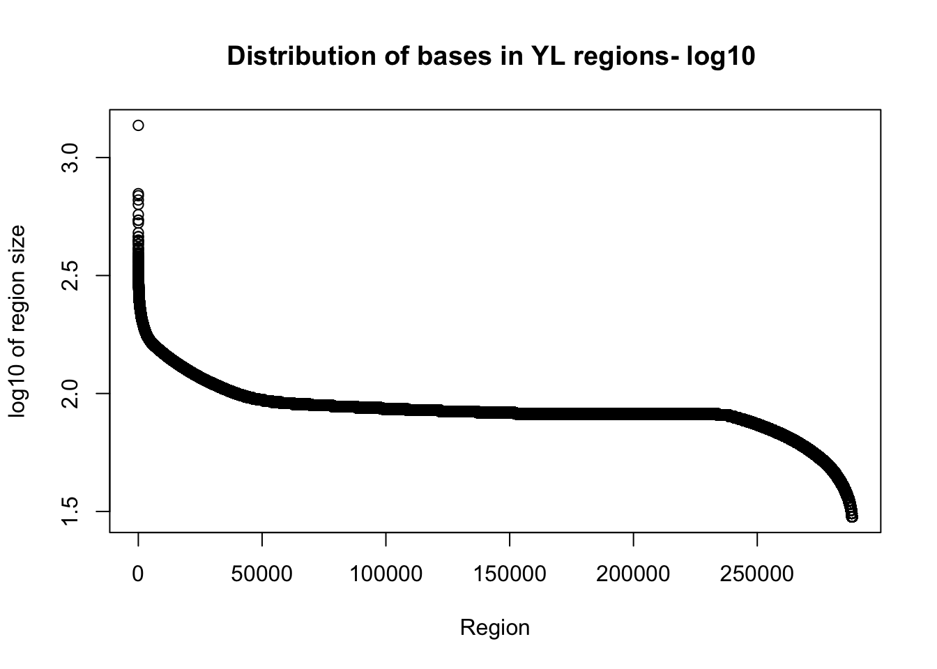
Expand here to see past versions of unnamed-chunk-26-1.png:
| Version | Author | Date |
|---|---|---|
| a0541e3 | Briana Mittleman | 2018-07-06 |
Plot number of bases against the mean:
YLplot=ggplot(YL_peaks, aes(y=log10(length), x=log10(count))) +
         geom_point(na.rm = TRUE, size = 0.1) +
         geom_density2d(na.rm = TRUE, size = 1, colour = 'red') +
         ylab('Log10 Region size') +
         xlab('Log10 Mean region coverage') +
        scale_y_continuous(limits = c(0, 3)) +
ggtitle("YL Peaks Combined Total Libraries")library(cowplot)Warning: package 'cowplot' was built under R version 3.4.3
Attaching package: 'cowplot'The following object is masked from 'package:ggplot2':
ggsaveplot_grid(splitplot, YLplot)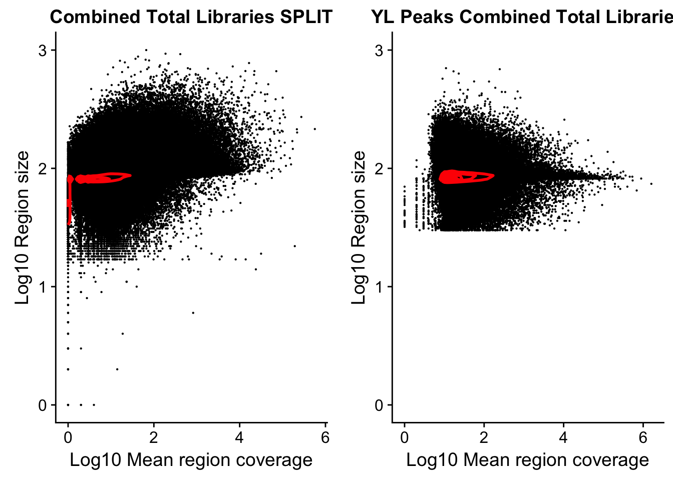
Expand here to see past versions of unnamed-chunk-28-1.png:
| Version | Author | Date |
|---|---|---|
| a0541e3 | Briana Mittleman | 2018-07-06 |
Run this on the Nuclear Fraction Bam
#!/bin/bash

#SBATCH --job-name=Ngencov_s
#SBATCH --account=pi-yangili1
#SBATCH --time=24:00:00
#SBATCH --output=Ngencov_s.out
#SBATCH --error=Ngencov_s.err
#SBATCH --partition=broadwl
#SBATCH --mem=40G
#SBATCH --mail-type=END


module load Anaconda3
source activate three-prime-env

samtools sort -o /project2/gilad/briana/threeprimeseq/data/macs2/NuclearBamFiles.sort.bam /project2/gilad/briana/threeprimeseq/data/macs2/NuclearBamFiles.bam


bedtools genomecov -ibam /project2/gilad/briana/threeprimeseq/data/macs2/NuclearBamFiles.sort.bam -d -split > /project2/gilad/briana/threeprimeseq/data/bedgraph/NuclearBamFiles.split.genomecov.bed
Session information
sessionInfo()R version 3.4.2 (2017-09-28)
Platform: x86_64-apple-darwin15.6.0 (64-bit)
Running under: macOS Sierra 10.12.6
Matrix products: default
BLAS: /Library/Frameworks/R.framework/Versions/3.4/Resources/lib/libRblas.0.dylib
LAPACK: /Library/Frameworks/R.framework/Versions/3.4/Resources/lib/libRlapack.dylib
locale:
[1] en_US.UTF-8/en_US.UTF-8/en_US.UTF-8/C/en_US.UTF-8/en_US.UTF-8
attached base packages:
[1] stats graphics grDevices utils datasets methods base
other attached packages:
[1] cowplot_0.9.2 bindrcpp_0.2.2 tidyr_0.7.2 workflowr_1.0.1
[5] rmarkdown_1.8.5 readr_1.1.1 ggplot2_2.2.1 dplyr_0.7.5
loaded via a namespace (and not attached):
[1] Rcpp_0.12.17 compiler_3.4.2 pillar_1.1.0
[4] git2r_0.21.0 plyr_1.8.4 bindr_0.1.1
[7] R.methodsS3_1.7.1 R.utils_2.6.0 tools_3.4.2
[10] digest_0.6.15 jsonlite_1.5 evaluate_0.10.1
[13] tibble_1.4.2 gtable_0.2.0 pkgconfig_2.0.1
[16] rlang_0.2.1 yaml_2.1.19 stringr_1.3.1
[19] knitr_1.18 hms_0.4.1 rprojroot_1.3-2
[22] grid_3.4.2 tidyselect_0.2.4 reticulate_1.4
[25] glue_1.2.0 R6_2.2.2 purrr_0.2.5
[28] magrittr_1.5 whisker_0.3-2 MASS_7.3-48
[31] backports_1.1.2 scales_0.5.0 htmltools_0.3.6
[34] assertthat_0.2.0 colorspace_1.3-2 labeling_0.3
[37] stringi_1.2.2 lazyeval_0.2.1 munsell_0.4.3
[40] R.oo_1.22.0
This reproducible R Markdown analysis was created with workflowr 1.0.1