initial_map_qc
Briana Mittleman
5/26/2018
Last updated: 2018-06-01
workflowr checks: (Click a bullet for more information)-
✔ R Markdown file: up-to-date
Great! Since the R Markdown file has been committed to the Git repository, you know the exact version of the code that produced these results.
-
✔ Environment: empty
Great job! The global environment was empty. Objects defined in the global environment can affect the analysis in your R Markdown file in unknown ways. For reproduciblity it’s best to always run the code in an empty environment.
-
✔ Seed:
set.seed(12345)The command
set.seed(12345)was run prior to running the code in the R Markdown file. Setting a seed ensures that any results that rely on randomness, e.g. subsampling or permutations, are reproducible. -
✔ Session information: recorded
Great job! Recording the operating system, R version, and package versions is critical for reproducibility.
-
Great! You are using Git for version control. Tracking code development and connecting the code version to the results is critical for reproducibility. The version displayed above was the version of the Git repository at the time these results were generated.✔ Repository version: e4baa3b
Note that you need to be careful to ensure that all relevant files for the analysis have been committed to Git prior to generating the results (you can usewflow_publishorwflow_git_commit). workflowr only checks the R Markdown file, but you know if there are other scripts or data files that it depends on. Below is the status of the Git repository when the results were generated:
Note that any generated files, e.g. HTML, png, CSS, etc., are not included in this status report because it is ok for generated content to have uncommitted changes.Ignored files: Ignored: .Rhistory Ignored: .Rproj.user/ Untracked files: Untracked: data/gene_cov/ Untracked: data/reads_mapped_three_prime_seq.csv Unstaged changes: Modified: analysis/cov200bpwind.Rmd Modified: code/Snakefile
Expand here to see past versions:
| File | Version | Author | Date | Message |
|---|---|---|---|---|
| Rmd | e4baa3b | Briana Mittleman | 2018-06-01 | compare star and subj |
| html | 7126988 | Briana Mittleman | 2018-05-26 | Build site. |
| Rmd | 252c548 | Briana Mittleman | 2018-05-26 | plot prop mapping with subjunc |
| html | b5cdd59 | Briana Mittleman | 2018-05-26 | Build site. |
| Rmd | 9a49459 | Briana Mittleman | 2018-05-26 | start map qc analysis |
I will use this analysis to look at initial mapping QC for the two mappers I am using.
library(workflowr)Loading required package: rmarkdownThis is workflowr version 1.0.1
Run ?workflowr for help getting startedlibrary(ggplot2)
library(tidyr)
library(reshape2)Warning: package 'reshape2' was built under R version 3.4.3
Attaching package: 'reshape2'The following object is masked from 'package:tidyr':
smithslibrary(dplyr)
Attaching package: 'dplyr'The following objects are masked from 'package:stats':
filter, lagThe following objects are masked from 'package:base':
intersect, setdiff, setequal, unionlibrary(cowplot)Warning: package 'cowplot' was built under R version 3.4.3
Attaching package: 'cowplot'The following object is masked from 'package:ggplot2':
ggsaveSubjunc
I created a csv with the number of reads, mapped reads, and proportion of reads mapped per library.
subj_map= read.csv("../data/reads_mapped_three_prime_seq.csv", header=TRUE, stringsAsFactors = FALSE)
subj_map$line=as.factor(subj_map$line)
subj_map$fraction=as.factor(subj_map$fraction)
Summaries for each number:
summary(subj_map$reads) Min. 1st Qu. Median Mean 3rd Qu. Max.
5103350 8030068 8776602 8670328 9341566 10931074 summary(subj_map$mapped) Min. 1st Qu. Median Mean 3rd Qu. Max.
3575191 5688940 6268228 6091626 6394260 7788593 summary(subj_map$prop_mapped) Min. 1st Qu. Median Mean 3rd Qu. Max.
0.6658 0.6932 0.7034 0.7025 0.7135 0.7343 Look at this graphically:
subj_melt=melt(subj_map, id.vars=c("line", "fraction"), measure.vars = c("reads", "mapped", "prop_mapped"))subj_prop_mapped= subj_melt %>% filter(variable=="prop_mapped")
subjplot=ggplot(subj_prop_mapped, aes(y=value, x=line, fill=fraction)) + geom_bar(stat="identity",position="dodge") + labs( title="Proportion of reads mapped with Subjunc") + ylab("Proportion mapped") + geom_hline(yintercept = mean(subj_prop_mapped$value)) + annotate("text",4, mean(subj_prop_mapped$value)- .1, vjust = -1, label = "Mean mapping proportion= .702")Star mapping
I added two lines to the csv file with the star map stats for each line.
star_map= read.csv("../data/reads_mapped_three_prime_seq.csv", header=TRUE, stringsAsFactors = FALSE)
star_map$line=as.factor(star_map$line)
star_map$fraction=as.factor(star_map$fraction)
Summaries for each number:
summary(star_map$star_mapped) Min. 1st Qu. Median Mean 3rd Qu. Max.
3326506 5426888 5868012 5834521 6314488 7814874 summary(star_map$star_prop_mapped) Min. 1st Qu. Median Mean 3rd Qu. Max.
0.5648 0.6452 0.6558 0.6719 0.7144 0.7827 Look at this graphically:
star_melt=melt(star_map, id.vars=c("line", "fraction"), measure.vars = c("reads", "star_mapped", "star_prop_mapped"))star_prop_mapped= star_melt %>% filter(variable=="star_prop_mapped")
starplot=ggplot(star_prop_mapped, aes(y=value, x=line, fill=fraction)) + geom_bar(stat="identity",position="dodge") + labs( title="Proportion of reads mapped with Star") + ylab("Proportion mapped") + geom_hline(yintercept = mean(star_prop_mapped$value)) + annotate("text",4, mean(star_prop_mapped$value)- .1, vjust = -1, label = "Mean mapping proportion= .672")Compare the plots:
plot_grid(subjplot,starplot)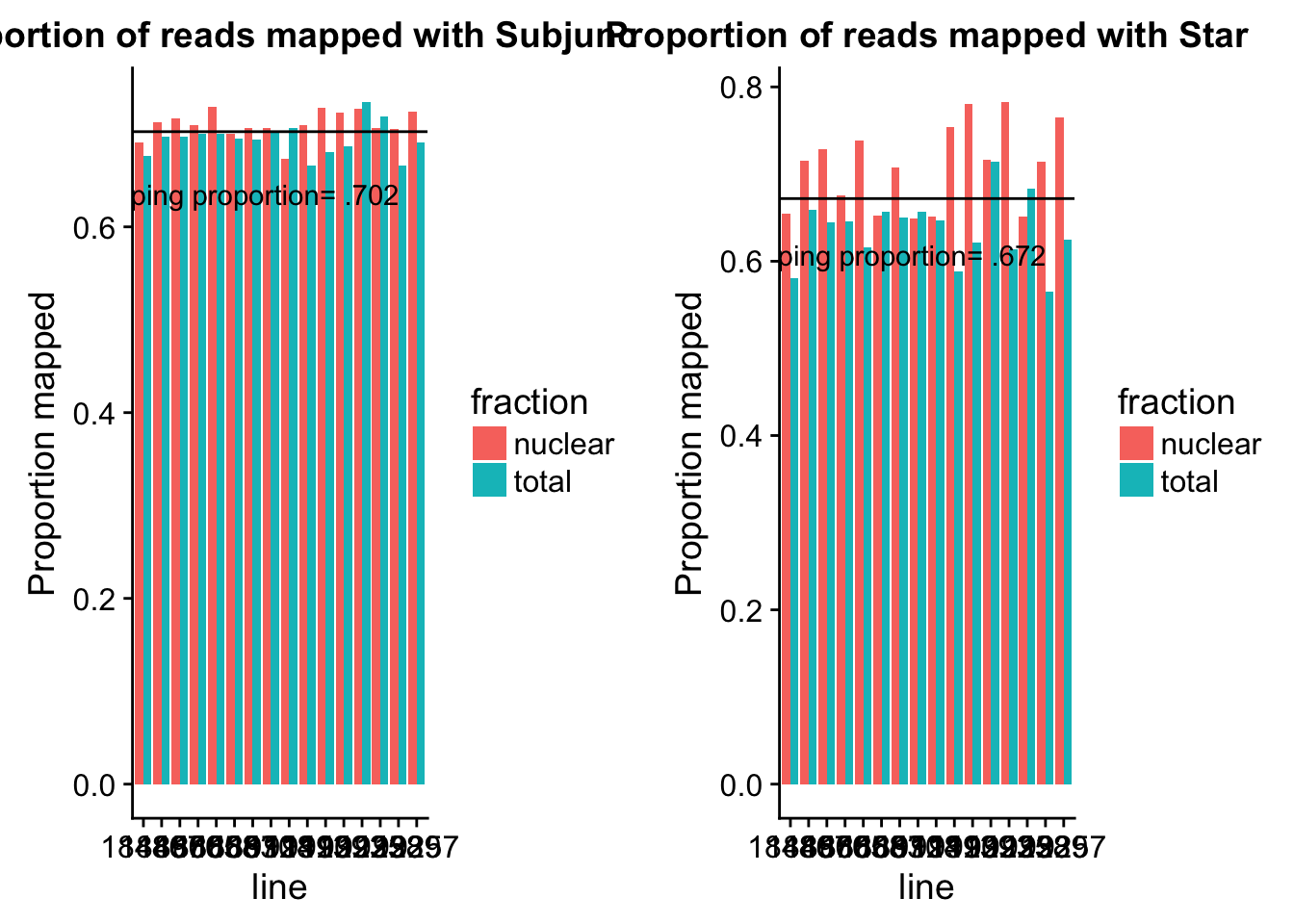
Session information
sessionInfo()R version 3.4.2 (2017-09-28)
Platform: x86_64-apple-darwin15.6.0 (64-bit)
Running under: macOS Sierra 10.12.6
Matrix products: default
BLAS: /Library/Frameworks/R.framework/Versions/3.4/Resources/lib/libRblas.0.dylib
LAPACK: /Library/Frameworks/R.framework/Versions/3.4/Resources/lib/libRlapack.dylib
locale:
[1] en_US.UTF-8/en_US.UTF-8/en_US.UTF-8/C/en_US.UTF-8/en_US.UTF-8
attached base packages:
[1] stats graphics grDevices utils datasets methods base
other attached packages:
[1] bindrcpp_0.2 cowplot_0.9.2 dplyr_0.7.4 reshape2_1.4.3
[5] tidyr_0.7.2 ggplot2_2.2.1 workflowr_1.0.1 rmarkdown_1.8.5
loaded via a namespace (and not attached):
[1] Rcpp_0.12.15 compiler_3.4.2 pillar_1.1.0
[4] git2r_0.21.0 plyr_1.8.4 bindr_0.1
[7] R.methodsS3_1.7.1 R.utils_2.6.0 tools_3.4.2
[10] digest_0.6.14 evaluate_0.10.1 tibble_1.4.2
[13] gtable_0.2.0 pkgconfig_2.0.1 rlang_0.1.6
[16] yaml_2.1.16 stringr_1.2.0 knitr_1.18
[19] rprojroot_1.3-2 grid_3.4.2 glue_1.2.0
[22] R6_2.2.2 purrr_0.2.4 magrittr_1.5
[25] whisker_0.3-2 backports_1.1.2 scales_0.5.0
[28] htmltools_0.3.6 assertthat_0.2.0 colorspace_1.3-2
[31] labeling_0.3 stringi_1.1.6 lazyeval_0.2.1
[34] munsell_0.4.3 R.oo_1.22.0
This reproducible R Markdown analysis was created with workflowr 1.0.1