Last updated: 2018-11-02

workflowr checks: (Click a bullet for more information)

✔ R Markdown file: up-to-date

Great! Since the R Markdown file has been committed to the Git repository, you know the exact version of the code that produced these results.
✔ Environment: empty

Great job! The global environment was empty. Objects defined in the global environment can affect the analysis in your R Markdown file in unknown ways. For reproduciblity it’s best to always run the code in an empty environment.
✔ Seed: set.seed(20181026)

The command set.seed(20181026) was run prior to running the code in the R Markdown file. Setting a seed ensures that any results that rely on randomness, e.g. subsampling or permutations, are reproducible.
✔ Session information: recorded

Great job! Recording the operating system, R version, and package versions is critical for reproducibility.
✔ Repository version: 97fa200
Great! You are using Git for version control. Tracking code development and connecting the code version to the results is critical for reproducibility. The version displayed above was the version of the Git repository at the time these results were generated.

Note that you need to be careful to ensure that all relevant files for the analysis have been committed to Git prior to generating the results (you can use wflow_publish or wflow_git_commit). workflowr only checks the R Markdown file, but you know if there are other scripts or data files that it depends on. Below is the status of the Git repository when the results were generated:
```
Unstaged changes:
    Modified:   plots/180504_alignment.pdf
    Modified:   plots/supplementary_figures/sfig_180504_alignment-discardedcells.pdf
    Modified:   plots/supplementary_figures/sfig_180504_biweightplots.pdf
```
Note that any generated files, e.g. HTML, png, CSS, etc., are not included in this status report because it is ok for generated content to have uncommitted changes.

Expand here to see past versions:

File	Version	Author	Date	Message
html	eaa7e4a	PytrikFolkertsma	2018-11-02	Build site.
Rmd	120215c	PytrikFolkertsma	2018-11-02	general analysis + alignment
html	120215c	PytrikFolkertsma	2018-11-02	general analysis + alignment
html	1f7e0da	PytrikFolkertsma	2018-10-30	Build site.
Rmd	f7080f1	PytrikFolkertsma	2018-10-30	wflow_publish(c(“analysis/10x-180504-general-analysis.Rmd”,

Analysis of the 10x samples: - tSNE plots - Cell cycle regression - PCA - Alignment - Marker gene expression - tSNE colored on metadata

Loading the required packages and datasets.

library(Seurat)

Loading required package: ggplot2

Loading required package: cowplot


Attaching package: 'cowplot'

The following object is masked from 'package:ggplot2':

    ggsave

Loading required package: Matrix

library(ggplot2)
library(dplyr)


Attaching package: 'dplyr'

The following objects are masked from 'package:stats':

    filter, lag

The following objects are masked from 'package:base':

    intersect, setdiff, setequal, union

all10x <- readRDS('output/10x-180504')
all10x.ccregout <- readRDS('output/10x-180504-ccregout')

QC Plots

VlnPlot(all10x, features.plot='nGene', group.by='sample_name', point.size.use=-1, x.lab.rot=T)

Expand here to see past versions of unnamed-chunk-2-1.png:

Version	Author	Date
1f7e0da	PytrikFolkertsma	2018-10-30

VlnPlot(all10x, features.plot='nUMI', group.by='sample_name', point.size.use=-1, x.lab.rot=T)

Expand here to see past versions of unnamed-chunk-3-1.png:

Version	Author	Date
1f7e0da	PytrikFolkertsma	2018-10-30

VlnPlot(all10x, features.plot='percent.mito', group.by='sample_name', point.size.use=-1, x.lab.rot=T)

Expand here to see past versions of unnamed-chunk-4-1.png:

Version	Author	Date
1f7e0da	PytrikFolkertsma	2018-10-30

GenePlot(all10x, 'nUMI', 'nGene')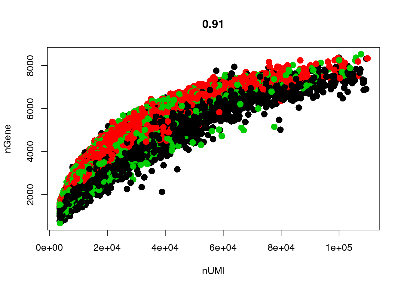

Expand here to see past versions of unnamed-chunk-5-1.png:

Version	Author	Date
1f7e0da	PytrikFolkertsma	2018-10-30

TSNE

Below are several tSNE plots of the 10x-180504 data. tSNE was performed on the first 15 principal components of the log-normalized scaled (nUMI and percent.mito regressed out) data.

Visceral and perirenal seem a bit mixed, and supraclavicular and subcutaneous too.

TSNEPlot(all10x, pt.size=0.1, group.by='sample_name', do.label=T)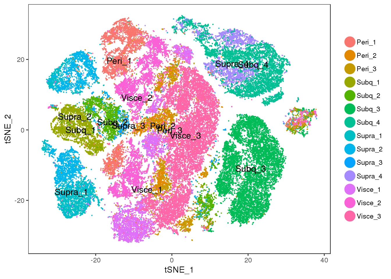

Expand here to see past versions of unnamed-chunk-6-1.png:

Version	Author	Date
1f7e0da	PytrikFolkertsma	2018-10-30

tSNE plots of samples within their depot. Peri2 and Peri3 seem to overlap really well, as well as Supra1 and Supra2, and Visce1 and Visce3.

plot_grid(t1, t2, t3, t4)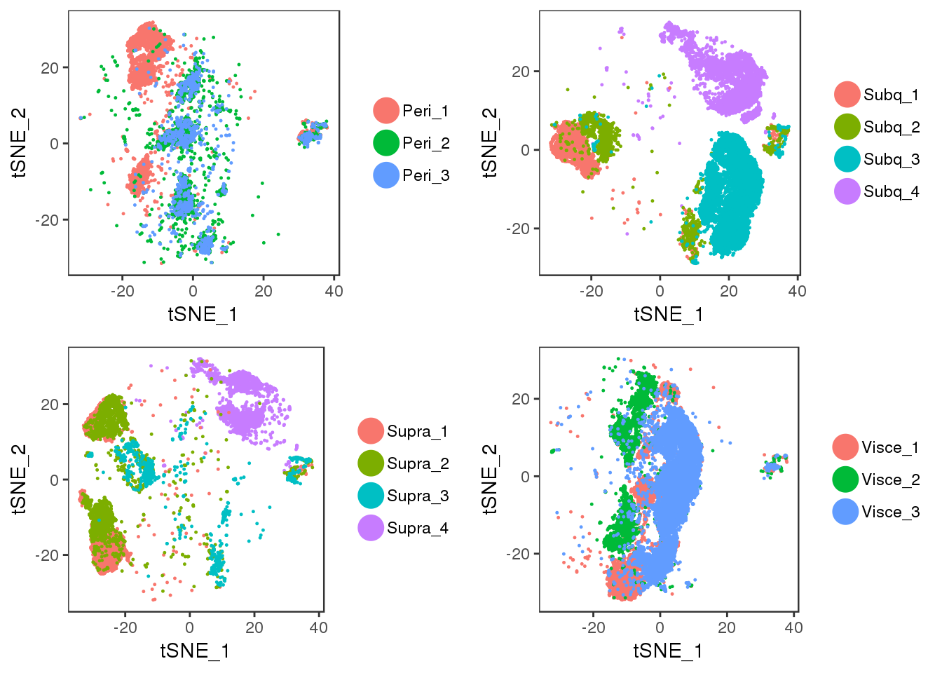

Expand here to see past versions of unnamed-chunk-8-1.png:

Version	Author	Date
1f7e0da	PytrikFolkertsma	2018-10-30

tSNE colored on subtissue.

TSNEPlot(all10x, group.by='depot', pt.size=0.1)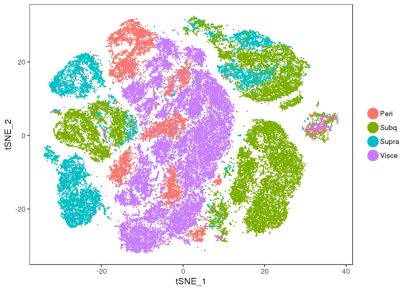

Expand here to see past versions of unnamed-chunk-9-1.png:

Version	Author	Date
1f7e0da	PytrikFolkertsma	2018-10-30

tSNE colored by cell cycle phase.

TSNEPlot(all10x, group.by='Phase', pt.size=0.1)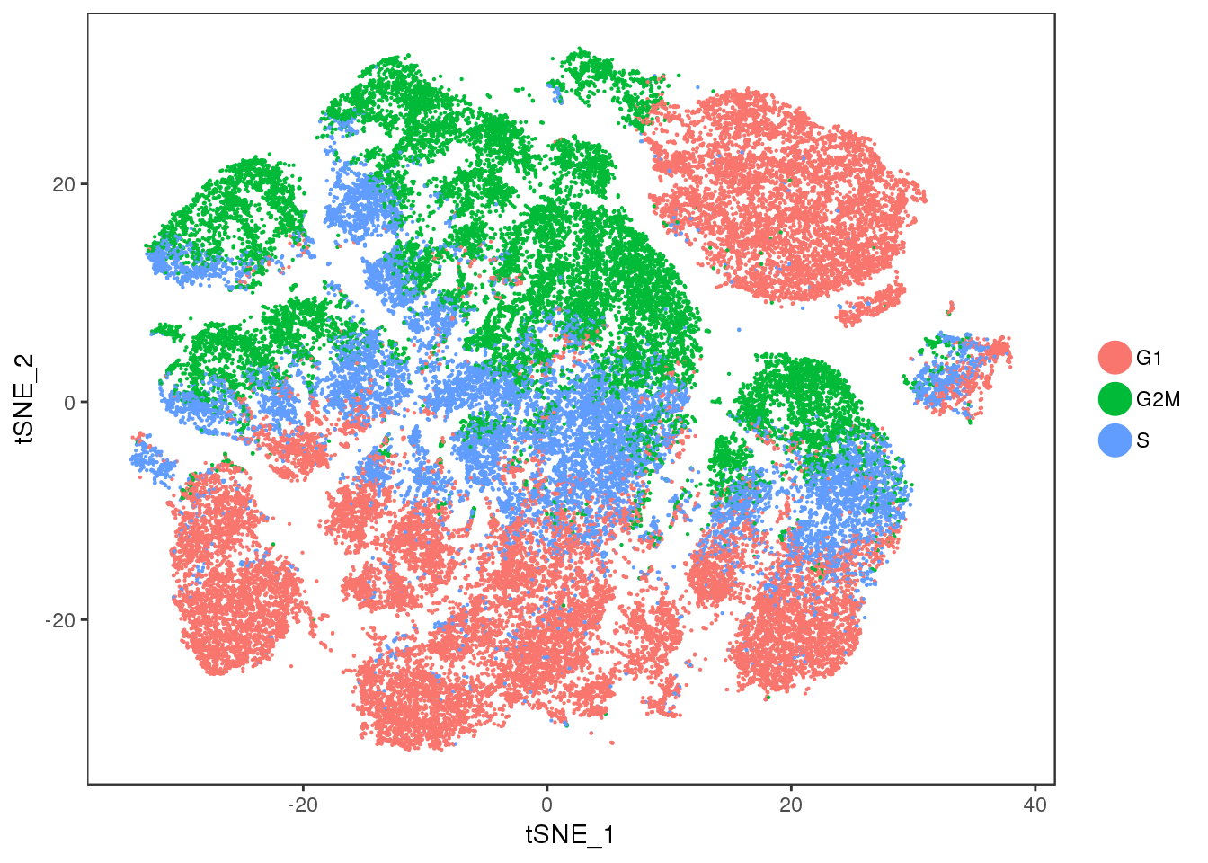

Expand here to see past versions of unnamed-chunk-10-1.png:

Version	Author	Date
1f7e0da	PytrikFolkertsma	2018-10-30

Clusters

Some clustering with different resolutions. res=0.5

TSNEPlot(all10x, pt.size=0.1, group.by='res.0.5', do.label=T)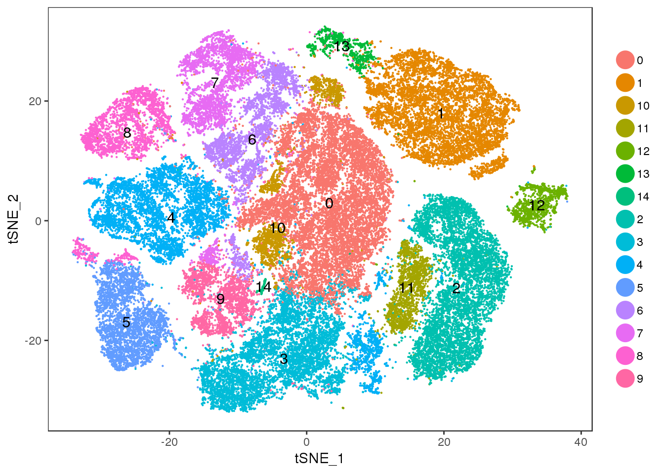

Expand here to see past versions of unnamed-chunk-11-1.png:

Version	Author	Date
1f7e0da	PytrikFolkertsma	2018-10-30

res=0.7

TSNEPlot(all10x, pt.size=0.1, group.by='res.0.7', do.label=T)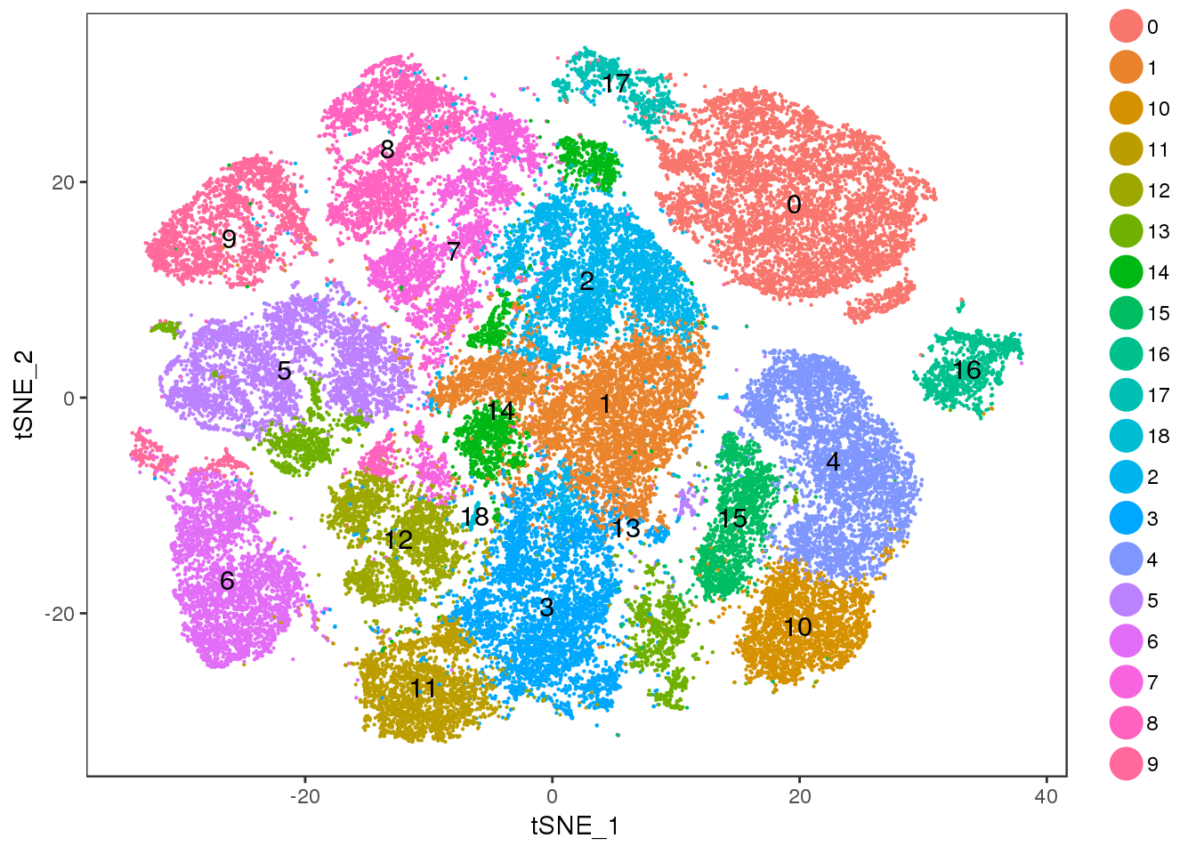

Expand here to see past versions of unnamed-chunk-12-1.png:

Version	Author	Date
1f7e0da	PytrikFolkertsma	2018-10-30

res=1

TSNEPlot(all10x, pt.size=0.1, group.by='res.1', do.label=T)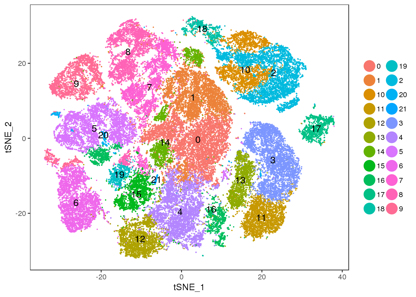

Expand here to see past versions of unnamed-chunk-13-1.png:

Version	Author	Date
1f7e0da	PytrikFolkertsma	2018-10-30

Cell cycle regression

T-SNE of the data with cell cycle effects regressed out. There does not seem to be a lot of structure within clusters now.

TSNEPlot(all10x.ccregout, pt.size=0.1, group.by='sample_name')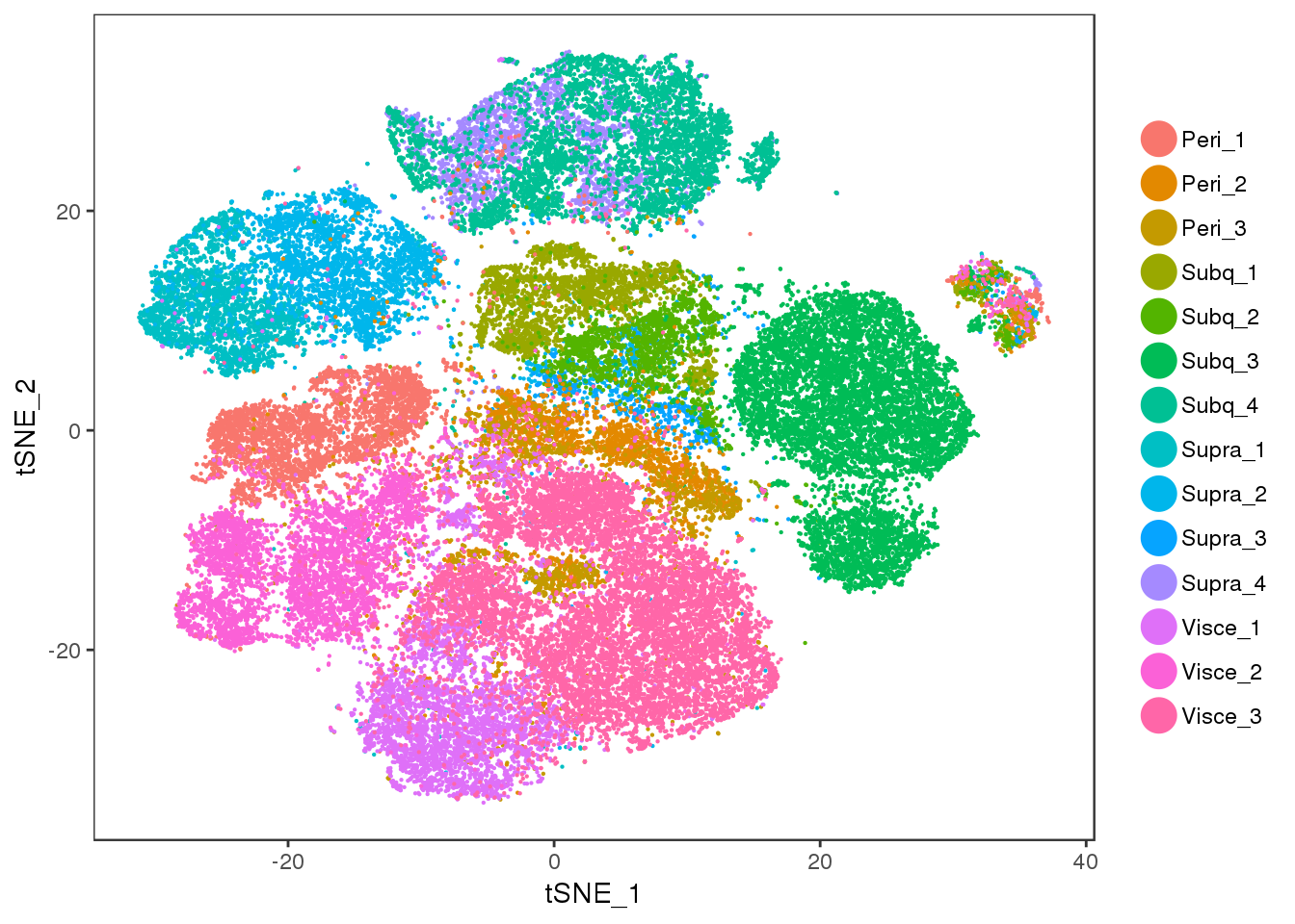

Expand here to see past versions of unnamed-chunk-14-1.png:

Version	Author	Date
120215c	PytrikFolkertsma	2018-11-02
1f7e0da	PytrikFolkertsma	2018-10-30

No cell cycle effect anymore.

TSNEPlot(all10x.ccregout, pt.size=0.1, group.by='Phase')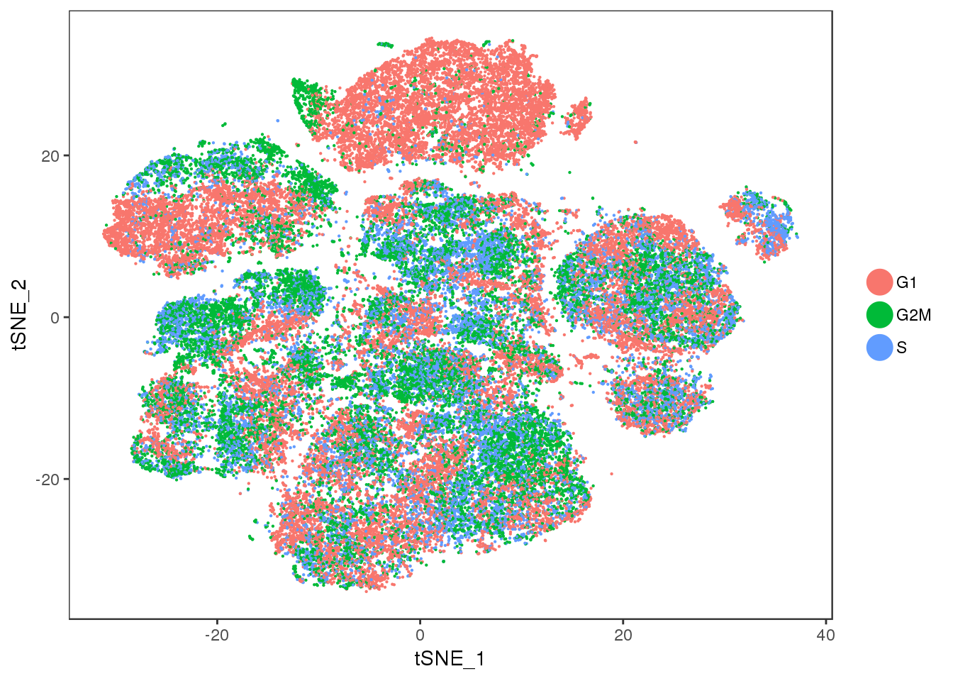

Expand here to see past versions of unnamed-chunk-15-1.png:

Version	Author	Date
120215c	PytrikFolkertsma	2018-11-02
1f7e0da	PytrikFolkertsma	2018-10-30

Subtissues

plot_grid(t1, t2, t3, t4)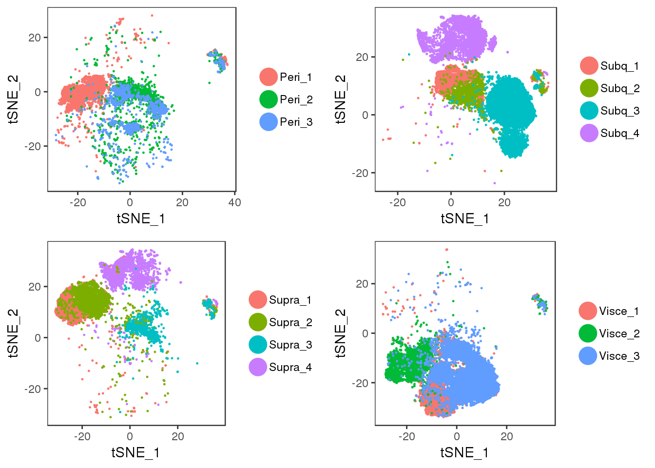

Expand here to see past versions of unnamed-chunk-17-1.png:

Version	Author	Date
120215c	PytrikFolkertsma	2018-11-02
1f7e0da	PytrikFolkertsma	2018-10-30

TSNEPlot(all10x.ccregout, pt.size=0.1, group.by='depot')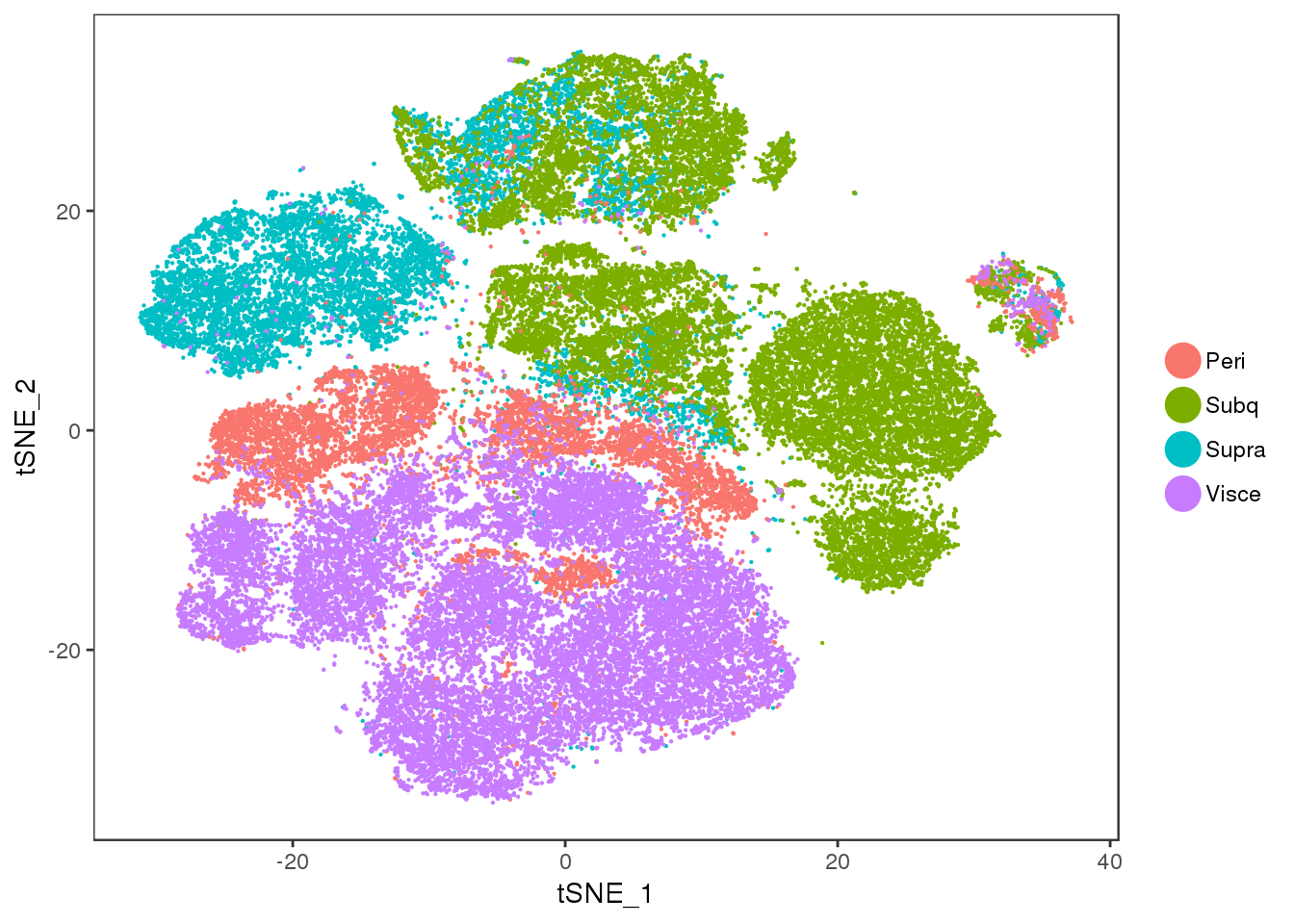

Expand here to see past versions of unnamed-chunk-18-1.png:

Version	Author	Date
120215c	PytrikFolkertsma	2018-11-02
1f7e0da	PytrikFolkertsma	2018-10-30

PCA

Some PCA plots. PC1 seems to capture cell cycle effects, and PC2 seems to capture some of the sample variability.

PCAPlot(all10x, group.by='Phase', pt.size=0.1)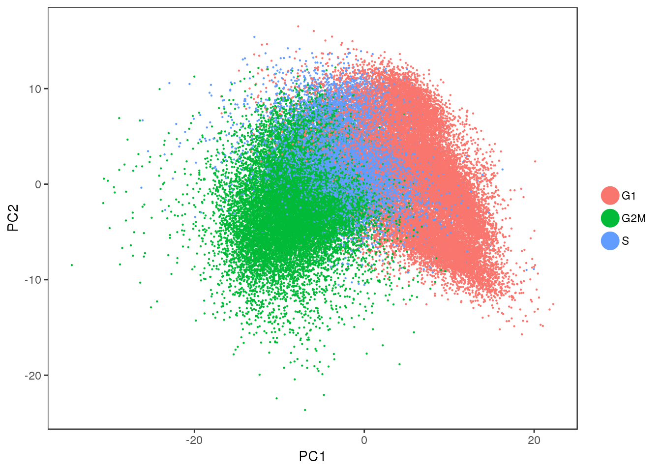

Expand here to see past versions of unnamed-chunk-19-1.png:

Version	Author	Date
120215c	PytrikFolkertsma	2018-11-02
1f7e0da	PytrikFolkertsma	2018-10-30

PCAPlot(all10x, group.by='sample_name', pt.size=0.1)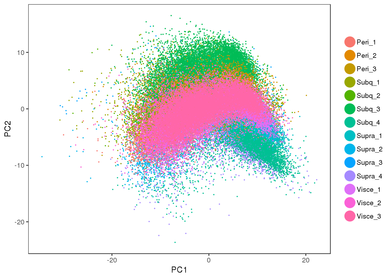

Expand here to see past versions of unnamed-chunk-20-1.png:

Version	Author	Date
120215c	PytrikFolkertsma	2018-11-02
1f7e0da	PytrikFolkertsma	2018-10-30

PCA plot of the cell cycle regressed out data. There is no cell cycle effect anymore.

PCAPlot(all10x.ccregout, group.by='Phase', pt.size=0.1)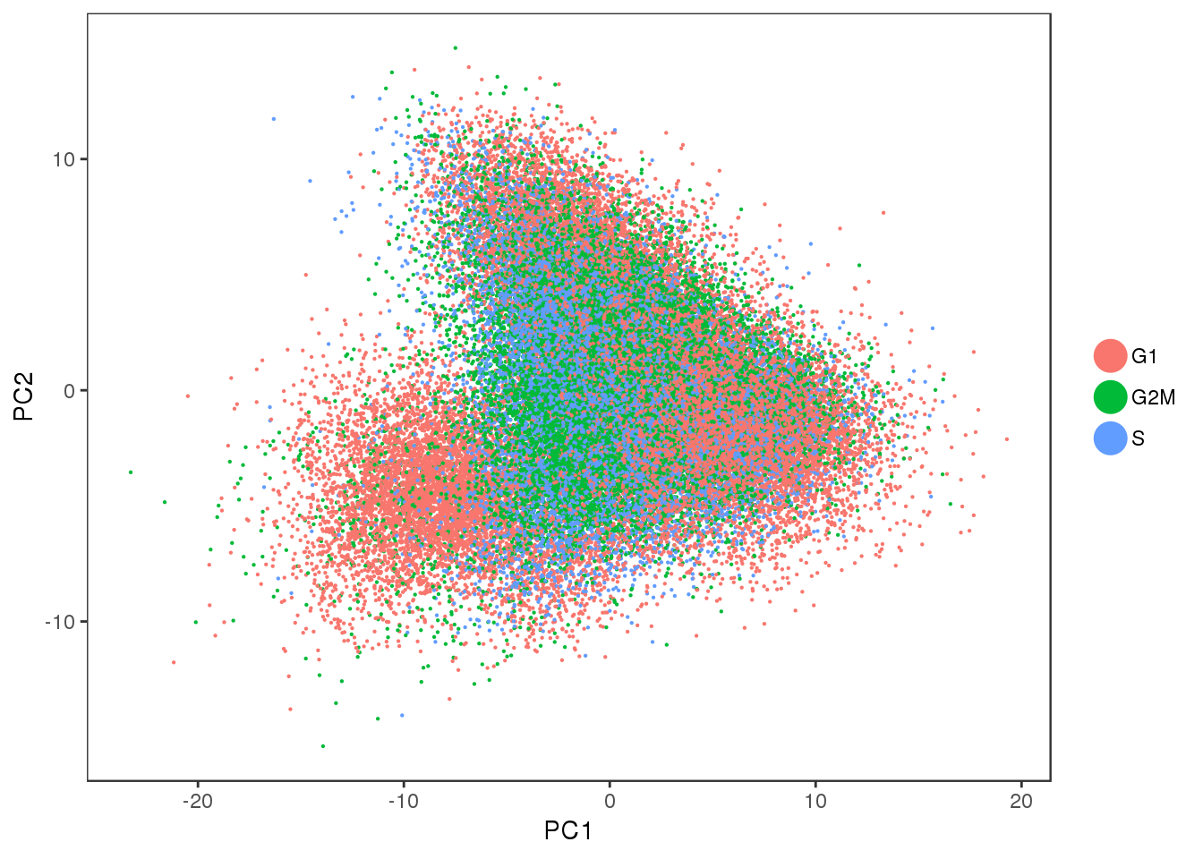

Expand here to see past versions of unnamed-chunk-21-1.png:

Version	Author	Date
120215c	PytrikFolkertsma	2018-11-02
1f7e0da	PytrikFolkertsma	2018-10-30

PCAPlot(all10x.ccregout, group.by='sample_name', pt.size=0.1)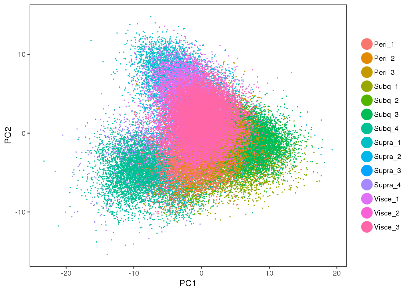

Expand here to see past versions of unnamed-chunk-22-1.png:

Version	Author	Date
120215c	PytrikFolkertsma	2018-11-02
1f7e0da	PytrikFolkertsma	2018-10-30

Metadata plots

FeaturePlot(all10x, c("nGene"), cols.use = c("grey","blue"), no.legend=F)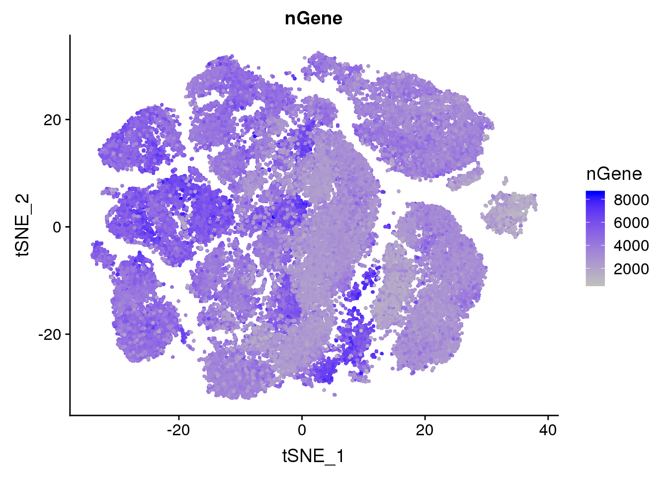

Expand here to see past versions of unnamed-chunk-23-1.png:

Version	Author	Date
120215c	PytrikFolkertsma	2018-11-02
1f7e0da	PytrikFolkertsma	2018-10-30

FeaturePlot(all10x, c("percent.mito"), cols.use = c("grey","blue"), no.legend=F)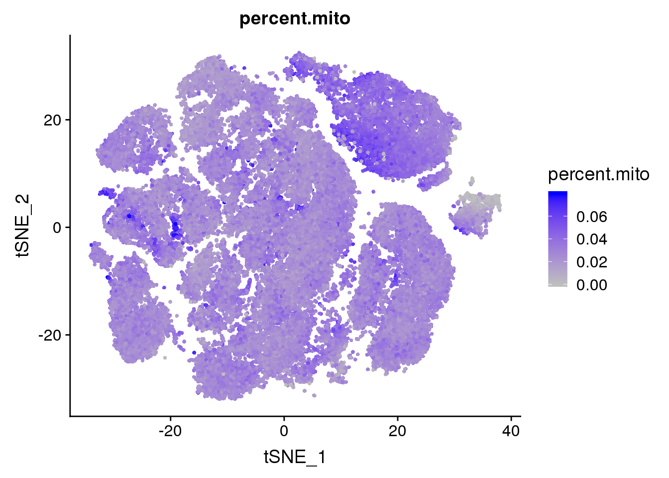

Expand here to see past versions of unnamed-chunk-24-1.png:

Version	Author	Date
120215c	PytrikFolkertsma	2018-11-02

FeaturePlot(all10x, c("nUMI"), cols.use = c("grey","blue"), no.legend=F)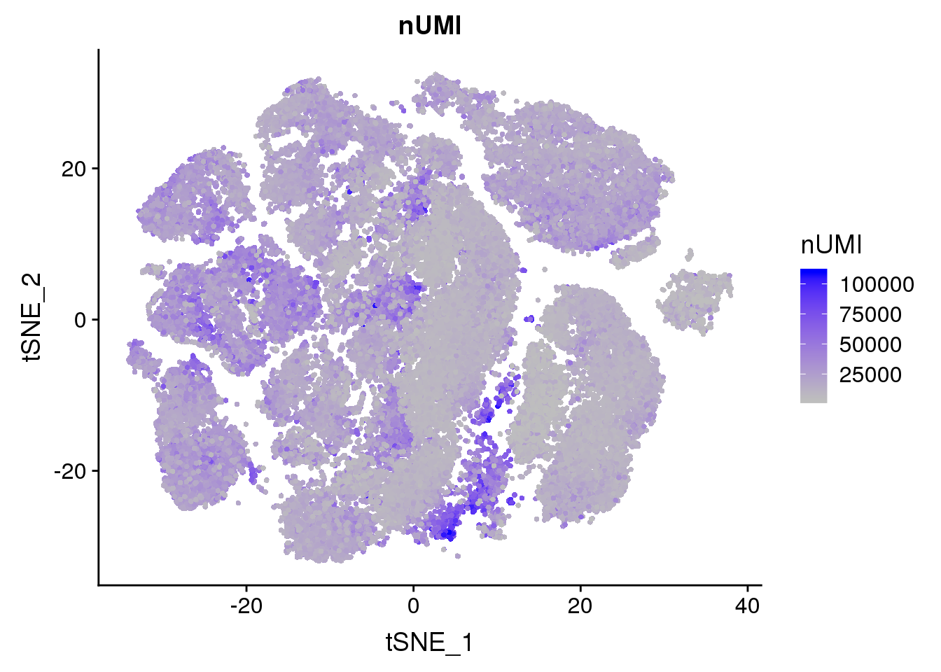

Expand here to see past versions of unnamed-chunk-25-1.png:

Version	Author	Date
120215c	PytrikFolkertsma	2018-11-02

Diff

TSNEPlot(all10x, group.by='diff', pt.size=0.1)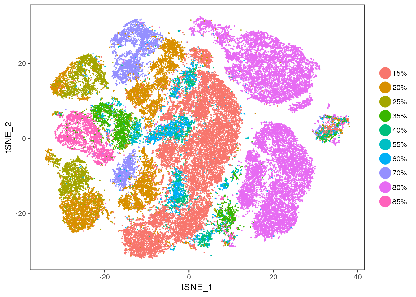

Expand here to see past versions of unnamed-chunk-26-1.png:

Version	Author	Date
120215c	PytrikFolkertsma	2018-11-02

all10x@meta.data['diff_int'] <- unlist(lapply(as.vector(unlist(all10x@meta.data$diff)), function(x){return(strtoi(strsplit(x, '%')))}))
FeaturePlot(all10x, features.plot='diff_int', cols.use=c('gray', 'blue'), no.legend=F)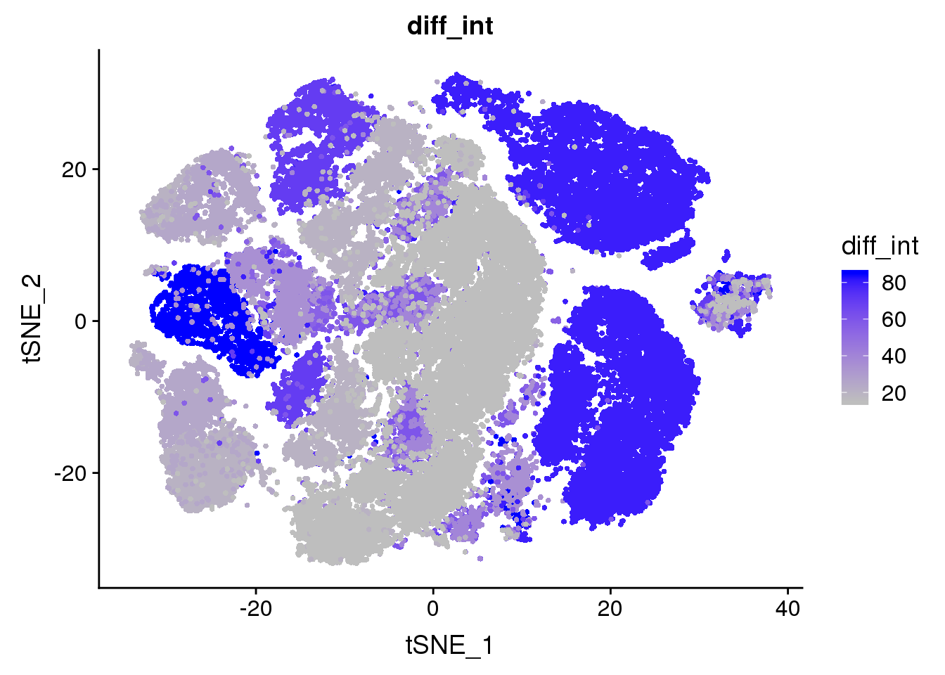

Expand here to see past versions of unnamed-chunk-27-1.png:

Version	Author	Date
120215c	PytrikFolkertsma	2018-11-02

ucp1.ctrl

TSNEPlot(all10x, group.by='ucp1.ctrl', pt.size=0.1)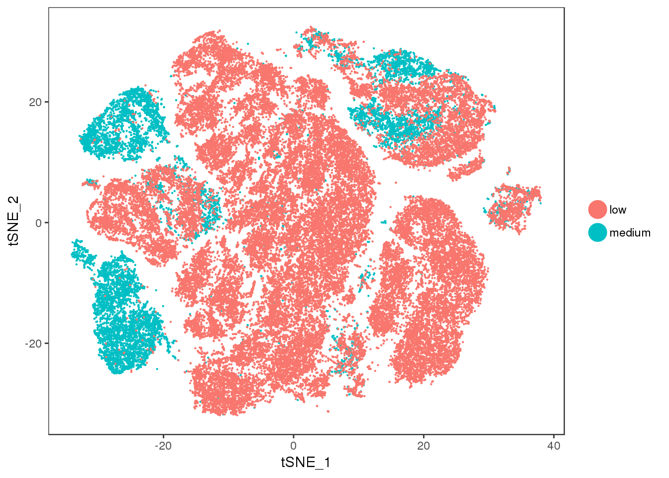

Expand here to see past versions of unnamed-chunk-28-1.png:

Version	Author	Date
120215c	PytrikFolkertsma	2018-11-02

ucp1.ne

TSNEPlot(all10x, group.by='ucp1.ne', pt.size=0.1)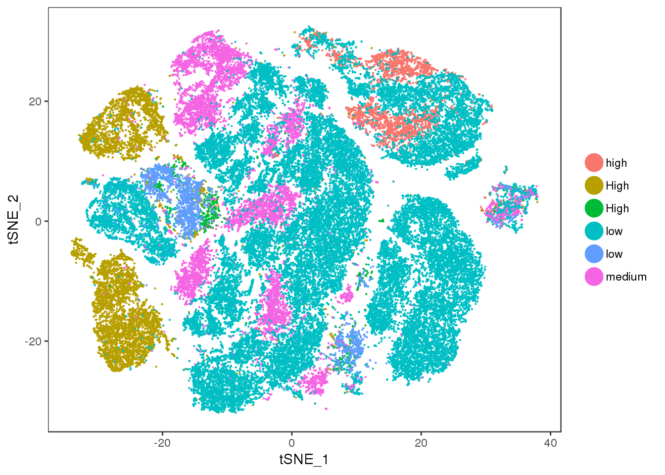

Expand here to see past versions of unnamed-chunk-29-1.png:

Version	Author	Date
120215c	PytrikFolkertsma	2018-11-02
1f7e0da	PytrikFolkertsma	2018-10-30

bmi

TSNEPlot(all10x, group.by='bmi', pt.size=0.1)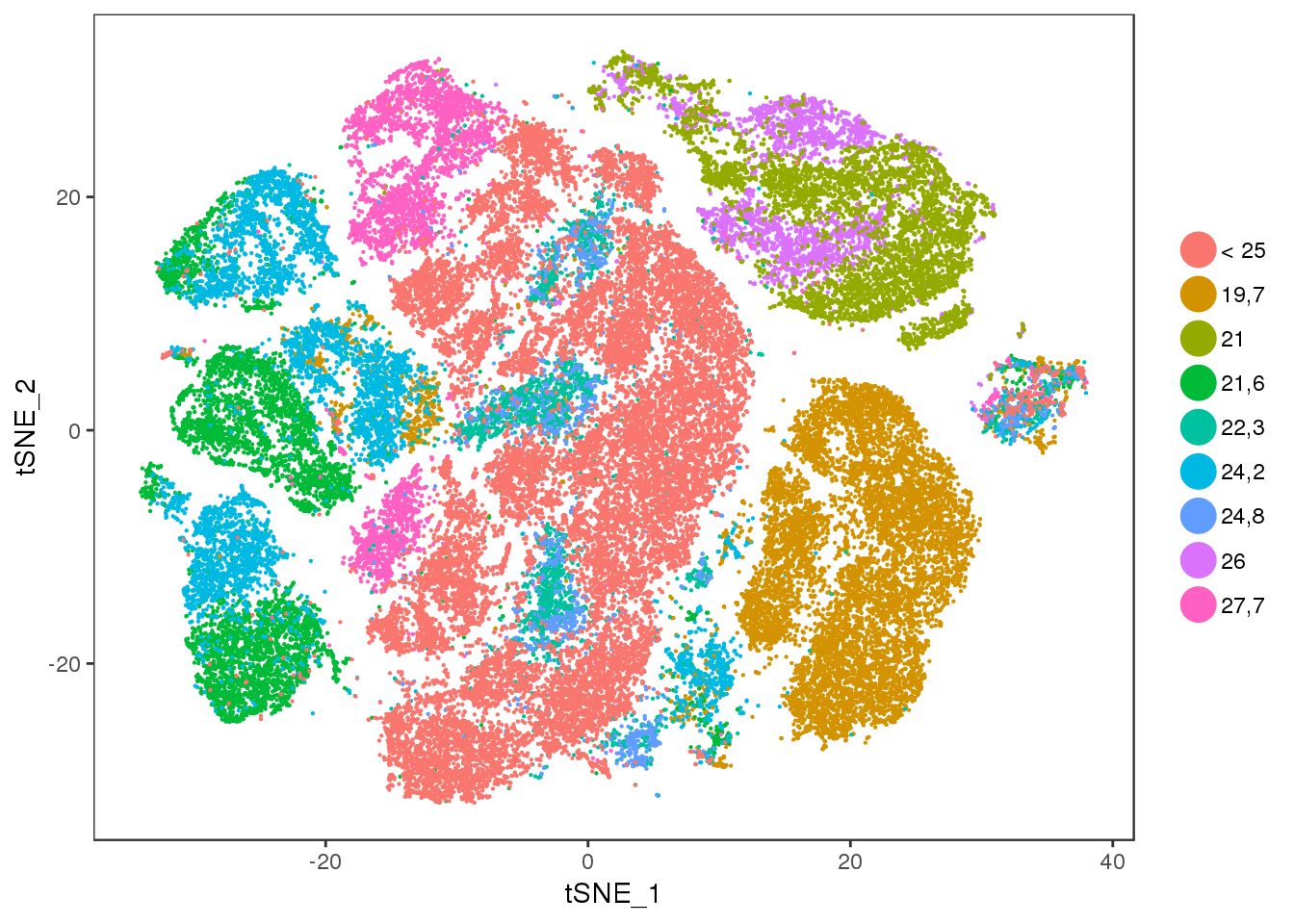

Expand here to see past versions of unnamed-chunk-30-1.png:

Version	Author	Date
120215c	PytrikFolkertsma	2018-11-02
1f7e0da	PytrikFolkertsma	2018-10-30

age

TSNEPlot(all10x, group.by='age', pt.size=0.1)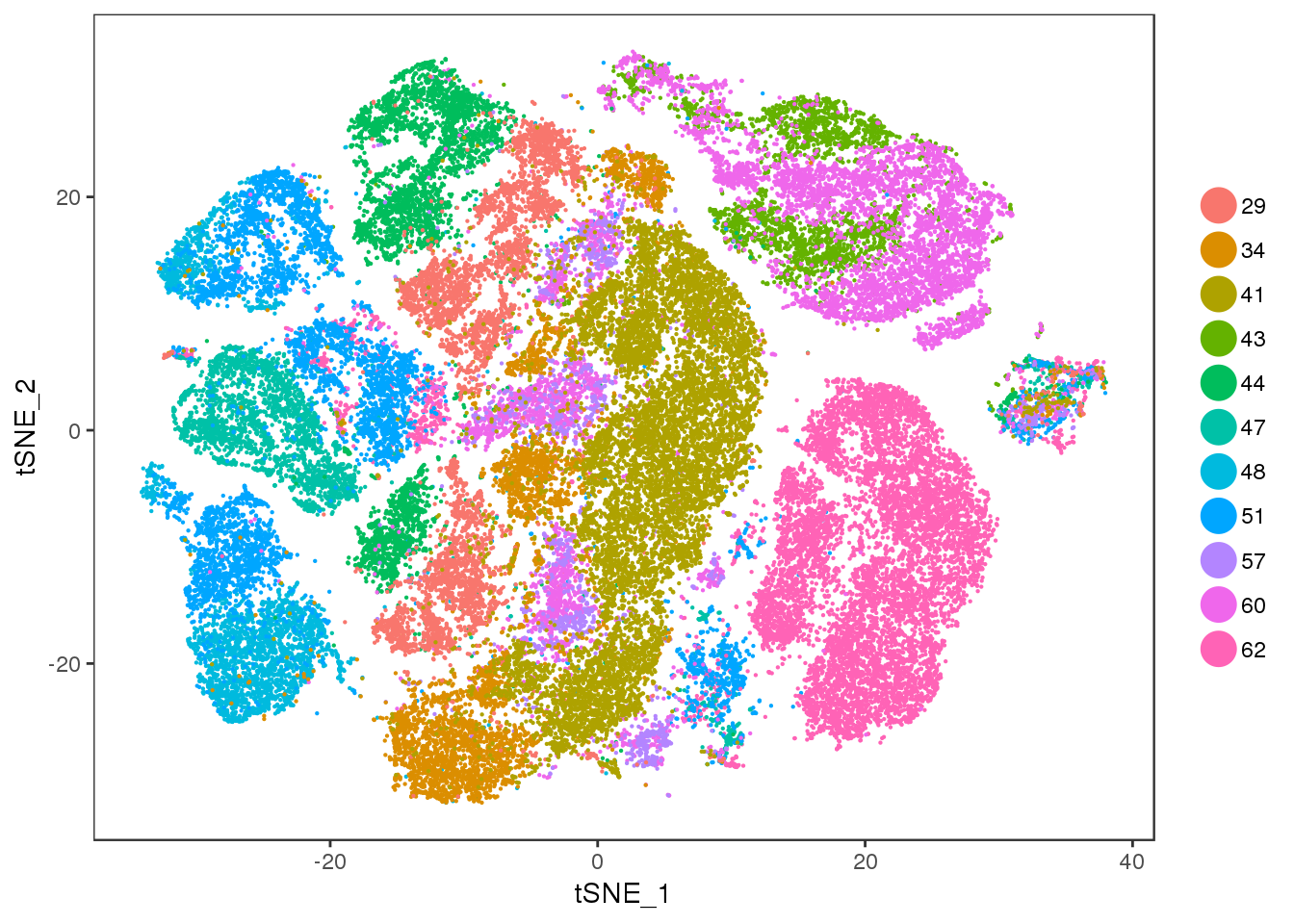

Expand here to see past versions of unnamed-chunk-31-1.png:

Version	Author	Date
120215c	PytrikFolkertsma	2018-11-02
1f7e0da	PytrikFolkertsma	2018-10-30

VlnPlot(all10x, group.by='sample_name', features.plot=c('nGene'), point.size.use = -1, x.lab.rot=T)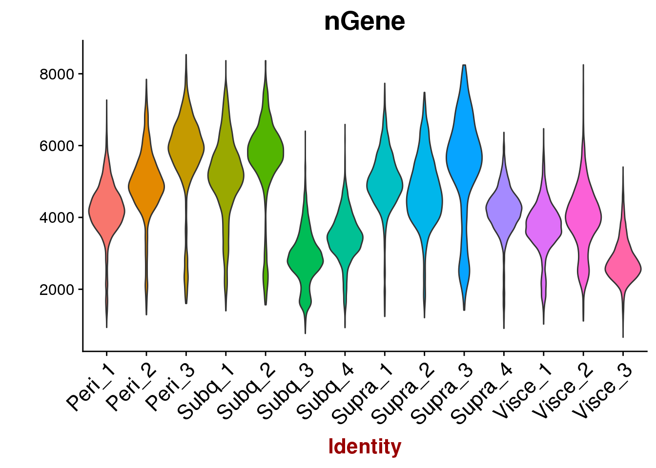

Expand here to see past versions of unnamed-chunk-32-1.png:

Version	Author	Date
120215c	PytrikFolkertsma	2018-11-02
1f7e0da	PytrikFolkertsma	2018-10-30

VlnPlot(all10x, group.by='sample_name', features.plot=c('nUMI'), point.size.use = -1, x.lab.rot=T)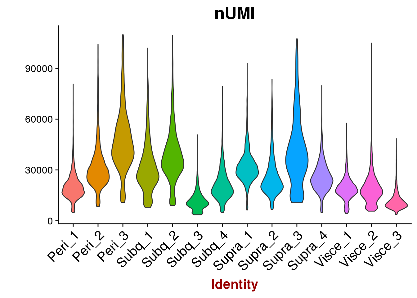

Expand here to see past versions of unnamed-chunk-33-1.png:

Version	Author	Date
120215c	PytrikFolkertsma	2018-11-02
1f7e0da	PytrikFolkertsma	2018-10-30

VlnPlot(all10x, group.by='sample_name', features.plot=c('percent.mito'), point.size.use = -1, x.lab.rot=T)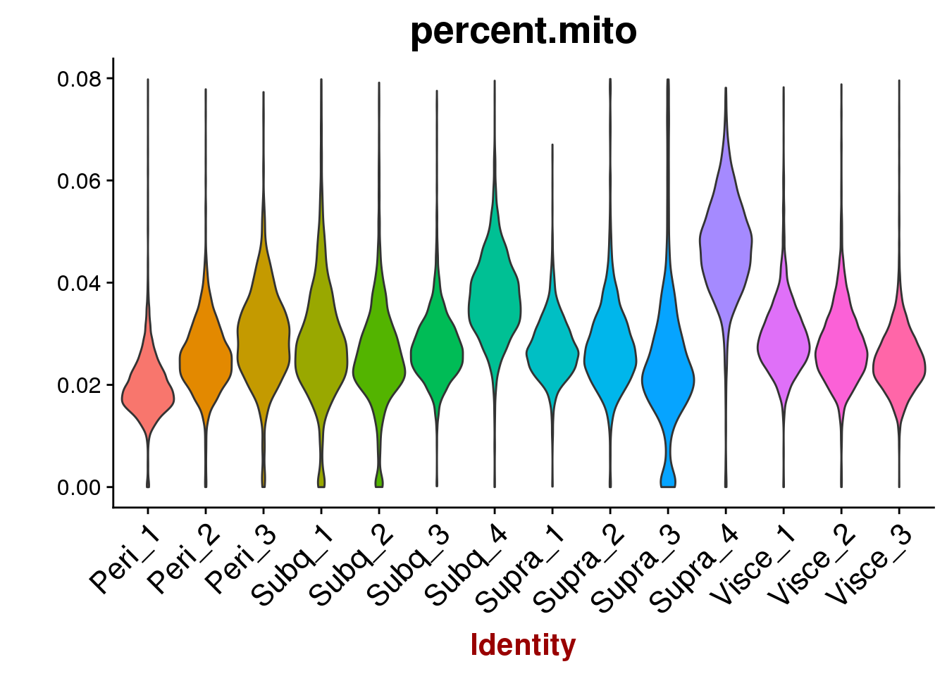

Expand here to see past versions of unnamed-chunk-34-1.png:

Version	Author	Date
120215c	PytrikFolkertsma	2018-11-02
1f7e0da	PytrikFolkertsma	2018-10-30

Mixture cluster 12

Sample composition in cluster 12.

cluster12 <- SubsetData(all10x, cells.use=rownames(all10x@meta.data)[which(all10x@meta.data$res.0.5 %in% 12)])
rotate_x <- function(data, column_to_plot, labels_vec, rot_angle) {
     plt <- barplot(data[[column_to_plot]], col='steelblue', xaxt="n")
     text(plt, par("usr")[3], labels = labels_vec, srt = rot_angle, adj = c(1.1,1.1), xpd = TRUE, cex=1)
}
rotate_x((cluster12@meta.data %>% count(sample_name))[,2], 'n', as.vector(unlist((cluster12@meta.data %>% count(sample_name))[,1])), 45)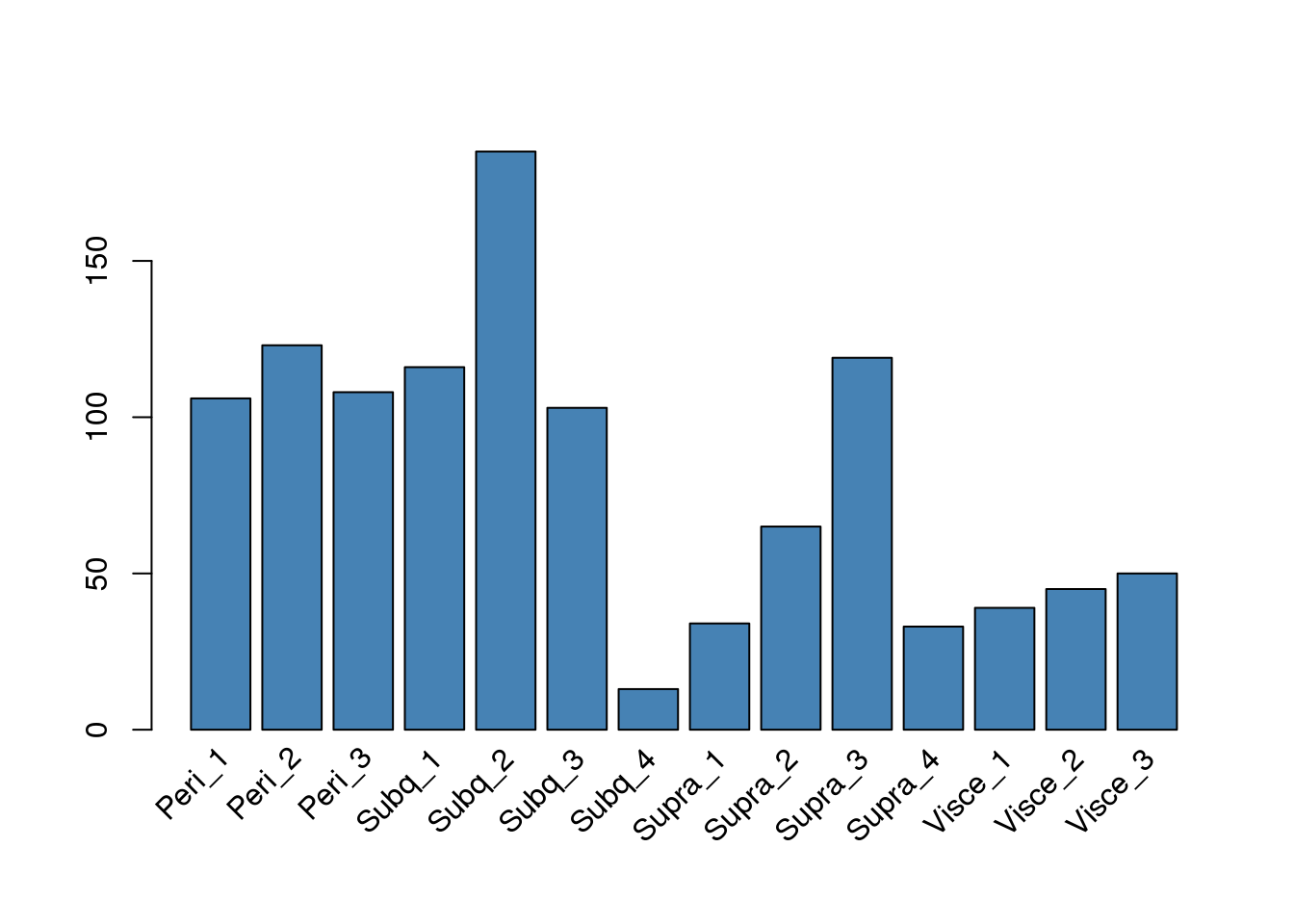

Expand here to see past versions of unnamed-chunk-35-1.png:

Version	Author	Date
120215c	PytrikFolkertsma	2018-11-02
1f7e0da	PytrikFolkertsma	2018-10-30

Figures for report

fig1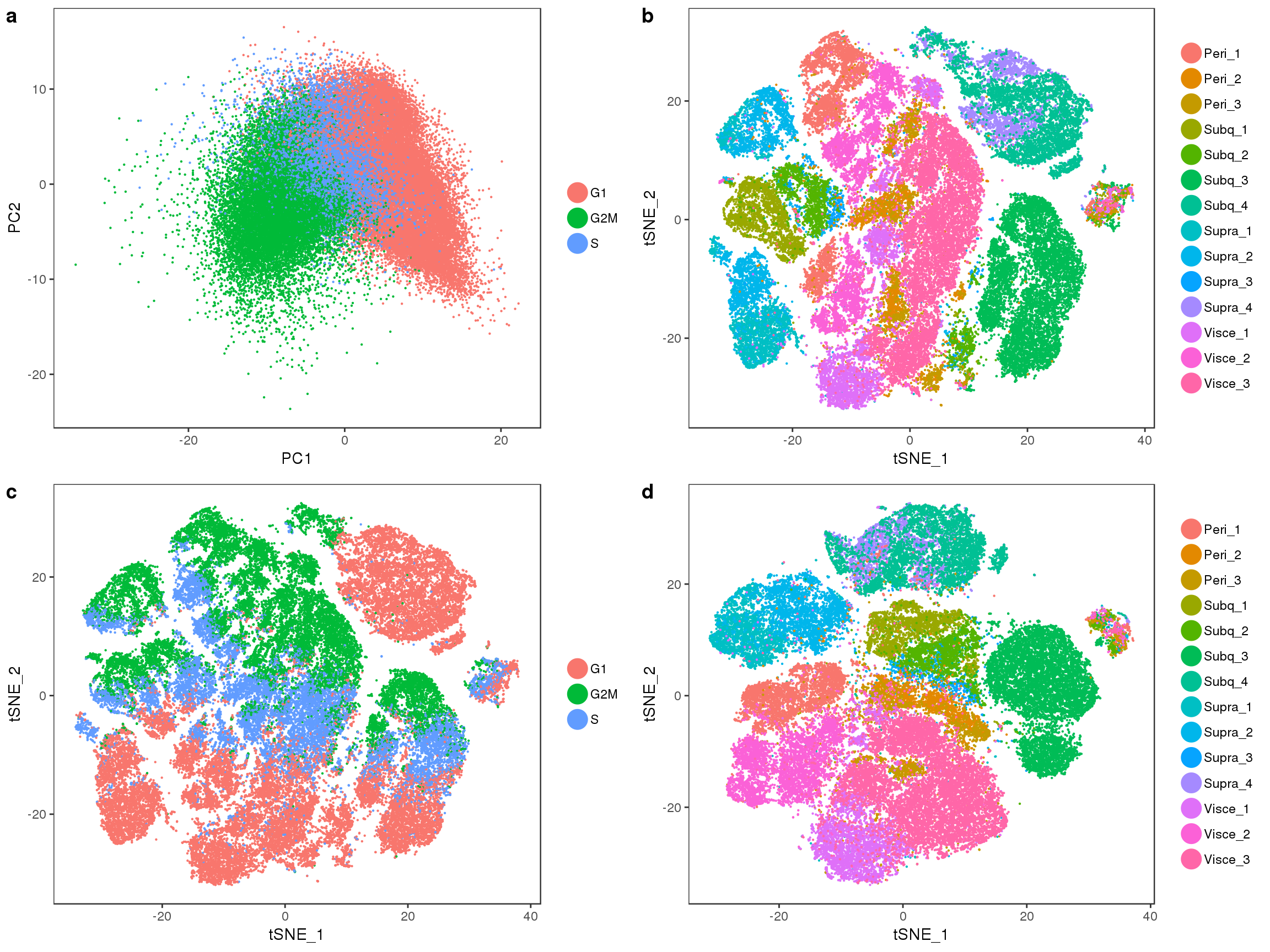

Expand here to see past versions of fig1-1.png:

Version	Author	Date
1f7e0da	PytrikFolkertsma	2018-10-30

#Supplementary figures
sfig1 <- plot_grid(
  VlnPlot(all10x, group.by='sample_name', features.plot=c('nGene'), point.size.use = -1, x.lab.rot=T, size.x.use=8),
  VlnPlot(all10x, group.by='sample_name', features.plot=c('nUMI'), point.size.use = -1, x.lab.rot=T, size.x.use=8),
  VlnPlot(all10x, group.by='sample_name', features.plot=c('percent.mito'), point.size.use = -1, x.lab.rot=T, size.x.use=8), 
  labels=c('a', 'b', 'c'), nrow=1
)
save_plot("plots/supplementary_figures/sfig_180504_qcplots.pdf", sfig1, base_width=12, base_height=3)
sfig1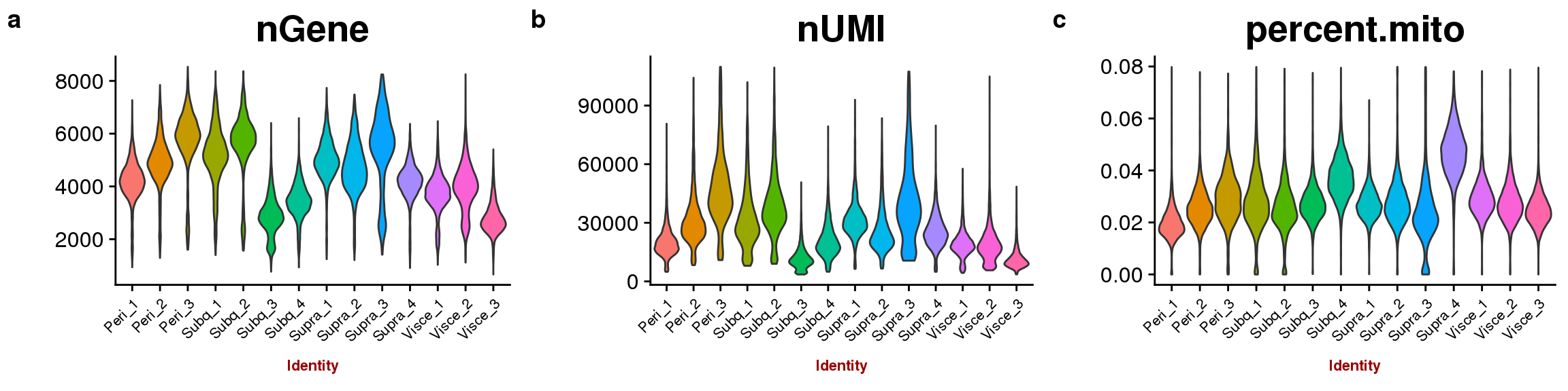

Expand here to see past versions of fig2-1.png:

Version	Author	Date
1f7e0da	PytrikFolkertsma	2018-10-30

sfig2 <- plot_grid(PCElbowPlot(all10x, num.pc=50))
save_plot("plots/supplementary_figures/sfig_180504_pcelbow.pdf", sfig2, base_width=8, base_height=5)
sfig2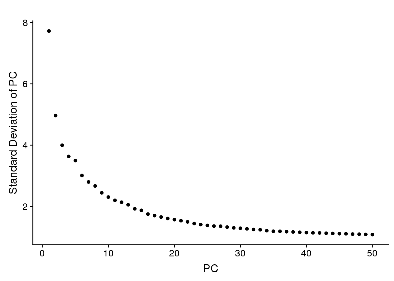

Expand here to see past versions of unnamed-chunk-37-1.png:

Version	Author	Date
120215c	PytrikFolkertsma	2018-11-02
1f7e0da	PytrikFolkertsma	2018-10-30

Session information

sessionInfo()

R version 3.4.3 (2017-11-30)
Platform: x86_64-redhat-linux-gnu (64-bit)
Running under: Red Hat Enterprise Linux

Matrix products: default
BLAS/LAPACK: /usr/lib64/R/lib/libRblas.so

locale:
 [1] LC_CTYPE=en_US.UTF-8       LC_NUMERIC=C              
 [3] LC_TIME=en_US.UTF-8        LC_COLLATE=en_US.UTF-8    
 [5] LC_MONETARY=en_US.UTF-8    LC_MESSAGES=en_US.UTF-8   
 [7] LC_PAPER=en_US.UTF-8       LC_NAME=C                 
 [9] LC_ADDRESS=C               LC_TELEPHONE=C            
[11] LC_MEASUREMENT=en_US.UTF-8 LC_IDENTIFICATION=C       

attached base packages:
[1] stats     graphics  grDevices utils     datasets  methods   base     

other attached packages:
[1] bindrcpp_0.2.2 dplyr_0.7.6    Seurat_2.3.4   Matrix_1.2-14 
[5] cowplot_0.9.3  ggplot2_3.0.0 

loaded via a namespace (and not attached):
  [1] Rtsne_0.13          colorspace_1.3-2    class_7.3-14       
  [4] modeltools_0.2-22   ggridges_0.5.0      mclust_5.4.1       
  [7] rprojroot_1.3-2     htmlTable_1.12      base64enc_0.1-3    
 [10] rstudioapi_0.7      proxy_0.4-22        flexmix_2.3-14     
 [13] bit64_0.9-7         mvtnorm_1.0-8       codetools_0.2-15   
 [16] splines_3.4.3       R.methodsS3_1.7.1   robustbase_0.93-2  
 [19] knitr_1.20          Formula_1.2-3       jsonlite_1.5       
 [22] workflowr_1.1.1     ica_1.0-2           cluster_2.0.7-1    
 [25] kernlab_0.9-27      png_0.1-7           R.oo_1.22.0        
 [28] compiler_3.4.3      httr_1.3.1          backports_1.1.2    
 [31] assertthat_0.2.0    lazyeval_0.2.1      lars_1.2           
 [34] acepack_1.4.1       htmltools_0.3.6     tools_3.4.3        
 [37] igraph_1.2.2        gtable_0.2.0        glue_1.3.0         
 [40] RANN_2.6            reshape2_1.4.3      Rcpp_0.12.18       
 [43] trimcluster_0.1-2.1 gdata_2.18.0        ape_5.1            
 [46] nlme_3.1-137        iterators_1.0.10    fpc_2.1-11.1       
 [49] gbRd_0.4-11         lmtest_0.9-36       stringr_1.3.1      
 [52] irlba_2.3.2         gtools_3.8.1        DEoptimR_1.0-8     
 [55] MASS_7.3-50         zoo_1.8-3           scales_1.0.0       
 [58] doSNOW_1.0.16       parallel_3.4.3      RColorBrewer_1.1-2 
 [61] yaml_2.2.0          reticulate_1.10     pbapply_1.3-4      
 [64] gridExtra_2.3       rpart_4.1-13        segmented_0.5-3.0  
 [67] latticeExtra_0.6-28 stringi_1.2.4       foreach_1.4.4      
 [70] checkmate_1.8.5     caTools_1.17.1.1    bibtex_0.4.2       
 [73] Rdpack_0.9-0        SDMTools_1.1-221    rlang_0.2.2        
 [76] pkgconfig_2.0.2     dtw_1.20-1          prabclus_2.2-6     
 [79] bitops_1.0-6        evaluate_0.11       lattice_0.20-35    
 [82] ROCR_1.0-7          purrr_0.2.5         bindr_0.1.1        
 [85] labeling_0.3        htmlwidgets_1.2     bit_1.1-14         
 [88] tidyselect_0.2.4    plyr_1.8.4          magrittr_1.5       
 [91] R6_2.2.2            snow_0.4-2          gplots_3.0.1       
 [94] Hmisc_4.1-1         pillar_1.3.0        whisker_0.3-2      
 [97] foreign_0.8-70      withr_2.1.2         fitdistrplus_1.0-9 
[100] mixtools_1.1.0      survival_2.42-6     nnet_7.3-12        
[103] tsne_0.1-3          tibble_1.4.2        crayon_1.3.4       
[106] hdf5r_1.0.0         KernSmooth_2.23-15  rmarkdown_1.10     
[109] grid_3.4.3          data.table_1.11.4   git2r_0.23.0       
[112] metap_1.0           digest_0.6.15       diptest_0.75-7     
[115] tidyr_0.8.1         R.utils_2.7.0       stats4_3.4.3       
[118] munsell_0.5.0

This reproducible R Markdown analysis was created with workflowr 1.1.1

R Notebook