R Notebook
Last updated: 2018-11-02
workflowr checks: (Click a bullet for more information)-
✔ R Markdown file: up-to-date
Great! Since the R Markdown file has been committed to the Git repository, you know the exact version of the code that produced these results.
-
✔ Environment: empty
Great job! The global environment was empty. Objects defined in the global environment can affect the analysis in your R Markdown file in unknown ways. For reproduciblity it’s best to always run the code in an empty environment.
-
✔ Seed:
set.seed(20181026)The command
set.seed(20181026)was run prior to running the code in the R Markdown file. Setting a seed ensures that any results that rely on randomness, e.g. subsampling or permutations, are reproducible. -
✔ Session information: recorded
Great job! Recording the operating system, R version, and package versions is critical for reproducibility.
-
Great! You are using Git for version control. Tracking code development and connecting the code version to the results is critical for reproducibility. The version displayed above was the version of the Git repository at the time these results were generated.✔ Repository version: 97fa200
Note that you need to be careful to ensure that all relevant files for the analysis have been committed to Git prior to generating the results (you can usewflow_publishorwflow_git_commit). workflowr only checks the R Markdown file, but you know if there are other scripts or data files that it depends on. Below is the status of the Git repository when the results were generated:
Note that any generated files, e.g. HTML, png, CSS, etc., are not included in this status report because it is ok for generated content to have uncommitted changes.working directory clean
Expand here to see past versions:
Notebook for alignment analsyis of the 180504 data.
library(Seurat)Loading required package: ggplot2Loading required package: cowplot
Attaching package: 'cowplot'The following object is masked from 'package:ggplot2':
ggsaveLoading required package: Matrixlibrary(ggplot2)load('output/10x-180504-aligned-metageneplot')
all10x.aligned <- readRDS('output/10x-180504-aligned')
all10x.aligned.ccregout <- readRDS('output/10x-180504-ccregout-aligned')
all10x.aligned.discardedcells <- readRDS('output/10x-180504-cca-discardedcells')
all10x.ccregout.aligned.discardedcells <- readRDS('output/10x-180504-ccregout-cca-discardedcells')Alignment of the data with and without cell cycle effects regressed out. Both were aligned on 30 subspaces, tSNE was performed on the first 15 CCs.
Shared correlation per CC
Normal alignment
p1`geom_smooth()` using method = 'loess' and formula 'y ~ x'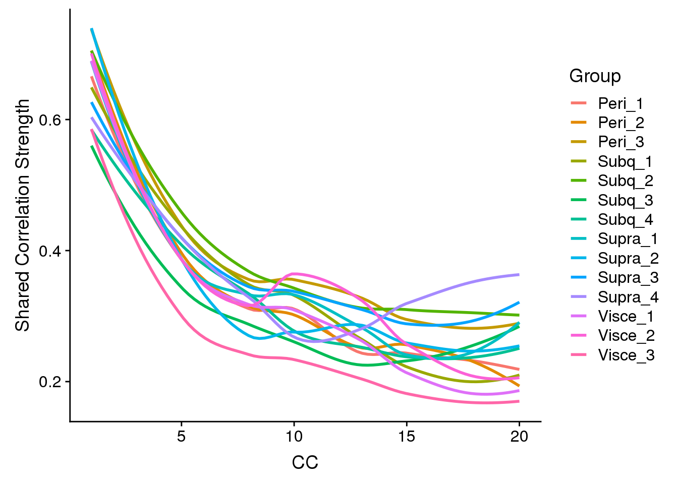
Expand here to see past versions of unnamed-chunk-3-1.png:
| Version | Author | Date |
|---|---|---|
| eaa7e4a | PytrikFolkertsma | 2018-11-02 |
Alignment with cell cycle effects regressed out
p2`geom_smooth()` using method = 'loess' and formula 'y ~ x'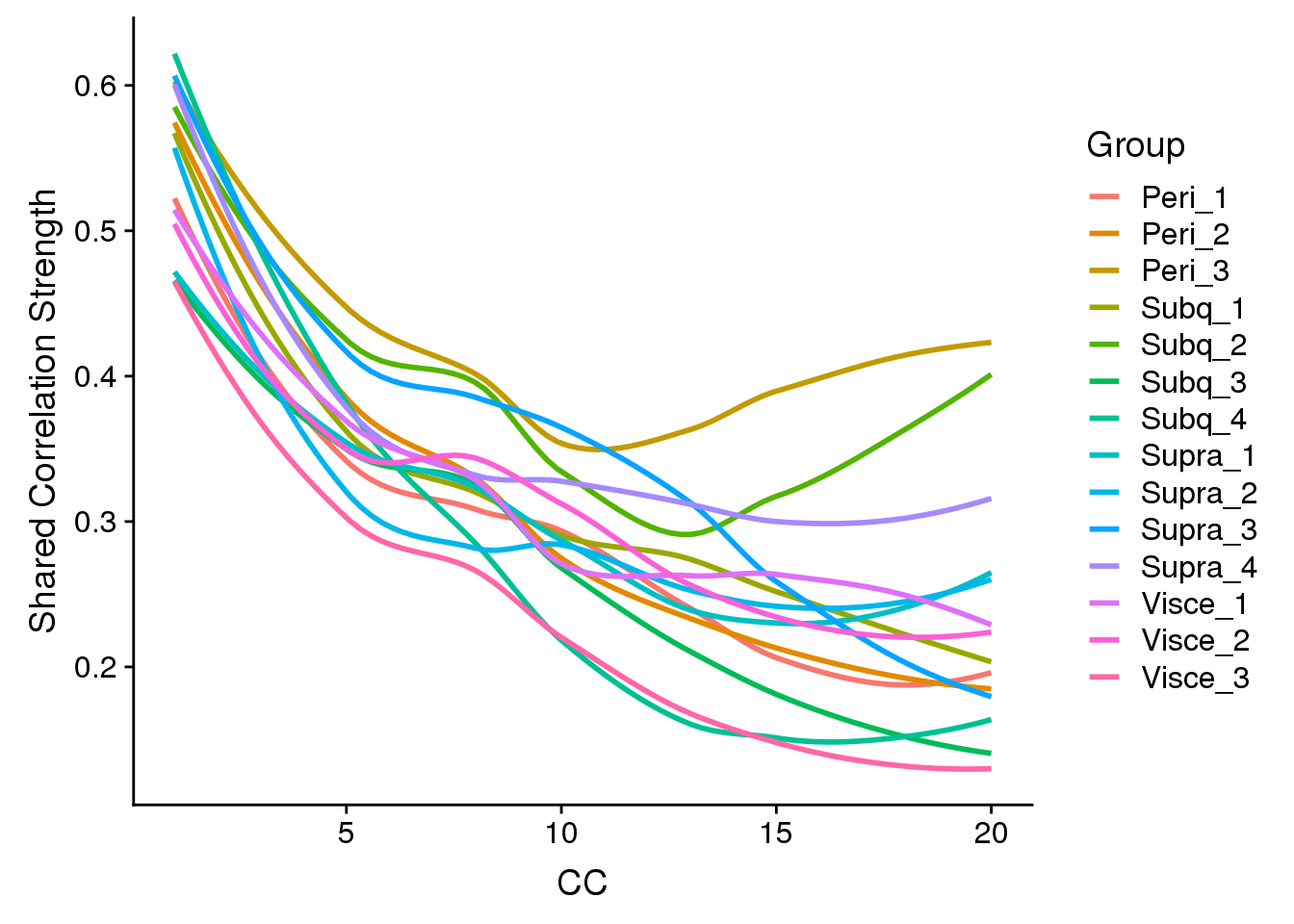
Expand here to see past versions of unnamed-chunk-4-1.png:
| Version | Author | Date |
|---|---|---|
| eaa7e4a | PytrikFolkertsma | 2018-11-02 |
Alignment without cell cycle effects regressed out
tSNE of the aligned data.
TSNEPlot(all10x.aligned, group.by='sample_name', pt.size=0.1)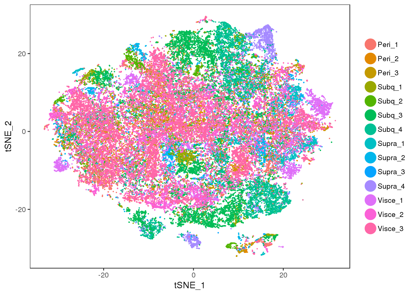
Expand here to see past versions of unnamed-chunk-5-1.png:
| Version | Author | Date |
|---|---|---|
| eaa7e4a | PytrikFolkertsma | 2018-11-02 |
tSNE of the aligned data coloured on cell cycle phase.
TSNEPlot(all10x.aligned, group.by='Phase', pt.size=0.1)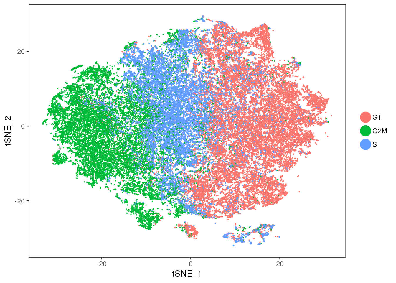
Expand here to see past versions of unnamed-chunk-6-1.png:
| Version | Author | Date |
|---|---|---|
| eaa7e4a | PytrikFolkertsma | 2018-11-02 |
Alignment with cell cycle regressed out
tSNE of the aligned data with cell cycle effects regressed out.
TSNEPlot(all10x.aligned.ccregout, group.by='sample_name', pt.size=0.1)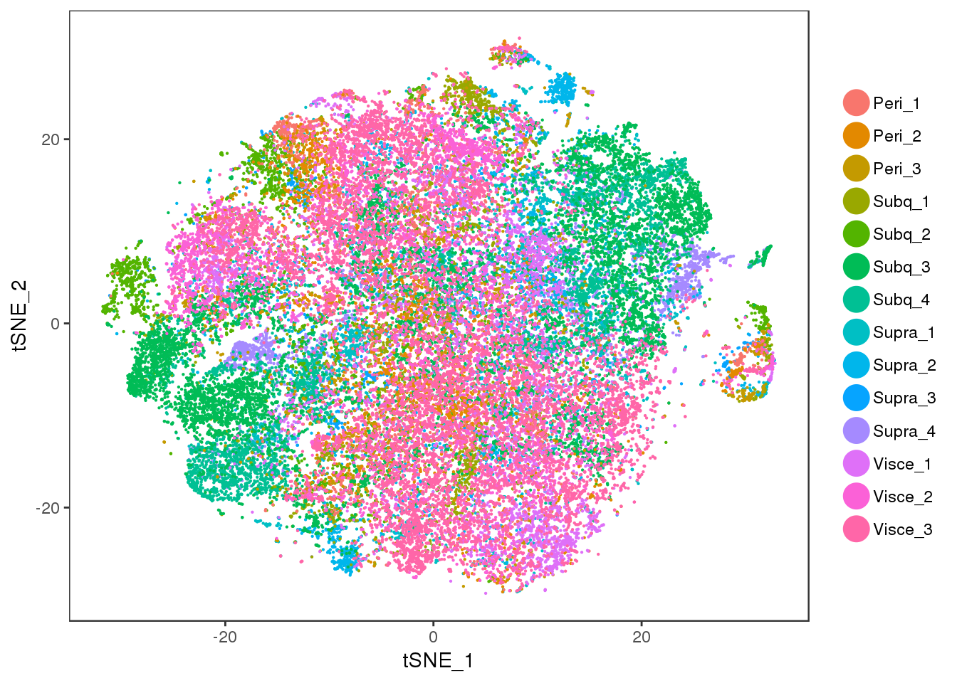
Expand here to see past versions of unnamed-chunk-7-1.png:
| Version | Author | Date |
|---|---|---|
| eaa7e4a | PytrikFolkertsma | 2018-11-02 |
tSNE of the aligned data with cell cycle effects regressed out, colored by phase.
TSNEPlot(all10x.aligned.ccregout, group.by='Phase', pt.size=0.1)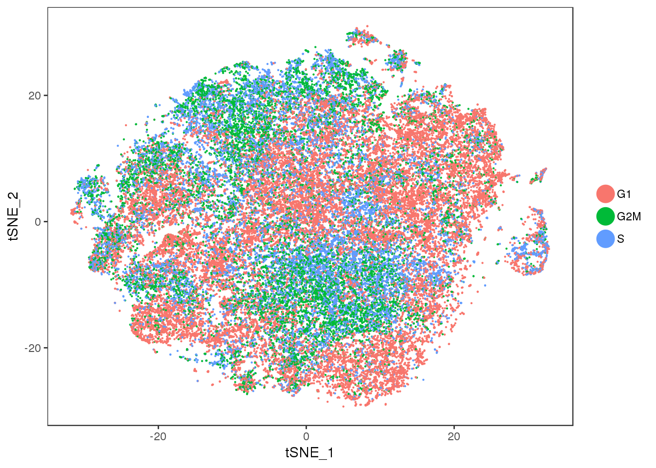
Expand here to see past versions of unnamed-chunk-8-1.png:
| Version | Author | Date |
|---|---|---|
| eaa7e4a | PytrikFolkertsma | 2018-11-02 |
tSNE of the aligned data with cell cycle effects regressed out, colored by subtissue
TSNEPlot(all10x.aligned.ccregout, group.by='depot', pt.size=0.1)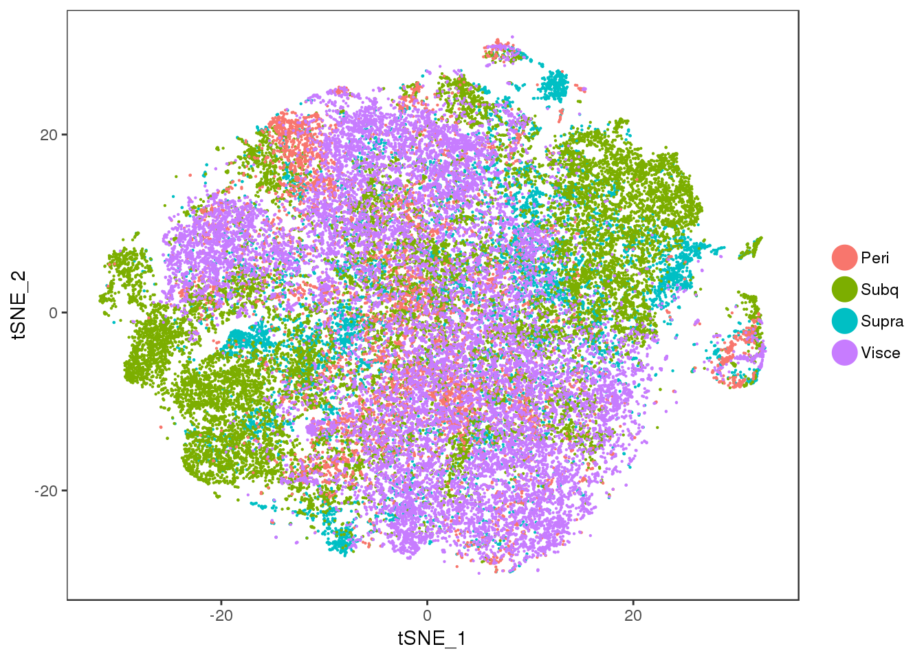
Expand here to see past versions of unnamed-chunk-9-1.png:
| Version | Author | Date |
|---|---|---|
| eaa7e4a | PytrikFolkertsma | 2018-11-02 |
Discarded cells from alignment
Before aligning the samples, sample-specific cells were discarded. Below: discarded cells from normal alignment.
discarded <- as.data.frame(table(all10x.aligned.discardedcells@meta.data$sample_name))

names(discarded) <- c('Sample', 'Frequency')

p_discarded <-ggplot(data=discarded, aes(x=Sample, y=Frequency)) +
  geom_bar(stat="identity") +
  theme(axis.text.x = element_text(angle=45, hjust=1))

p_discarded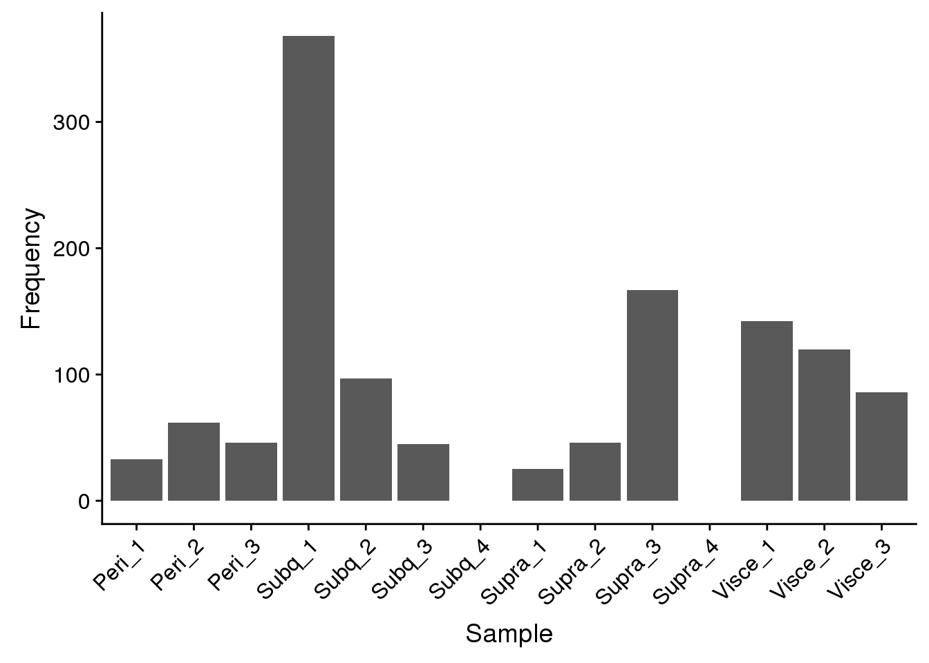
Expand here to see past versions of unnamed-chunk-10-1.png:
| Version | Author | Date |
|---|---|---|
| eaa7e4a | PytrikFolkertsma | 2018-11-02 |
Discarded cells from alignment with cell cycle effects regressed out.
discarded.ccregout <- as.data.frame(table(all10x.ccregout.aligned.discardedcells@meta.data$sample_name))

names(discarded.ccregout) <- c('Sample', 'Frequency')

p_discarded.ccregout <-ggplot(data=discarded.ccregout, aes(x=Sample, y=Frequency)) +
  geom_bar(stat="identity") +
  theme(axis.text.x = element_text(angle=45, hjust=1))

p_discarded.ccregout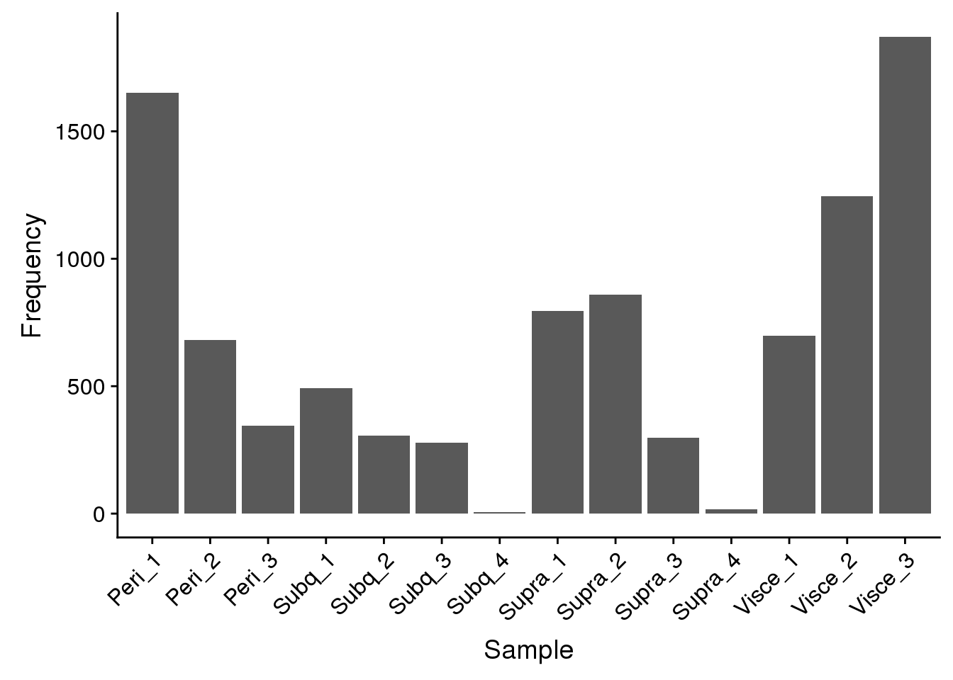
Expand here to see past versions of unnamed-chunk-11-1.png:
| Version | Author | Date |
|---|---|---|
| eaa7e4a | PytrikFolkertsma | 2018-11-02 |
Figures for report
fig1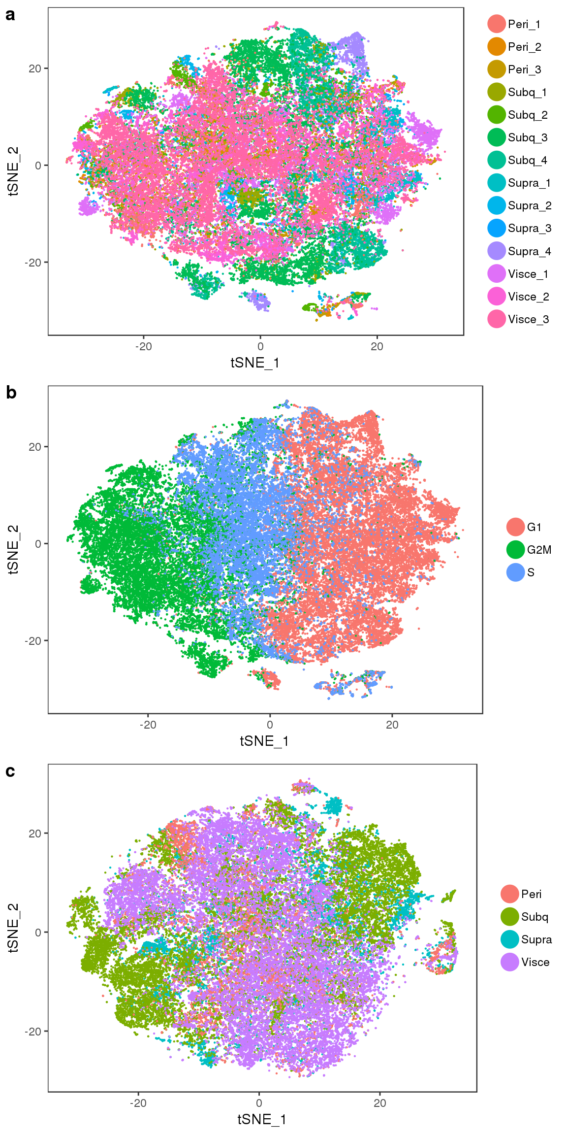
Expand here to see past versions of fig1-1.png:
| Version | Author | Date |
|---|---|---|
| eaa7e4a | PytrikFolkertsma | 2018-11-02 |
Biweight midcorrelation plots.
sfig1 <- plot_grid(
  p1,
  p2,
  labels=c('a', 'b'),
  nrow=1
)
`geom_smooth()` using method = 'loess' and formula 'y ~ x'
`geom_smooth()` using method = 'loess' and formula 'y ~ x'save_plot("plots/supplementary_figures/sfig_180504_biweightplots.pdf", sfig1, base_width=12, base_height=4)
sfig1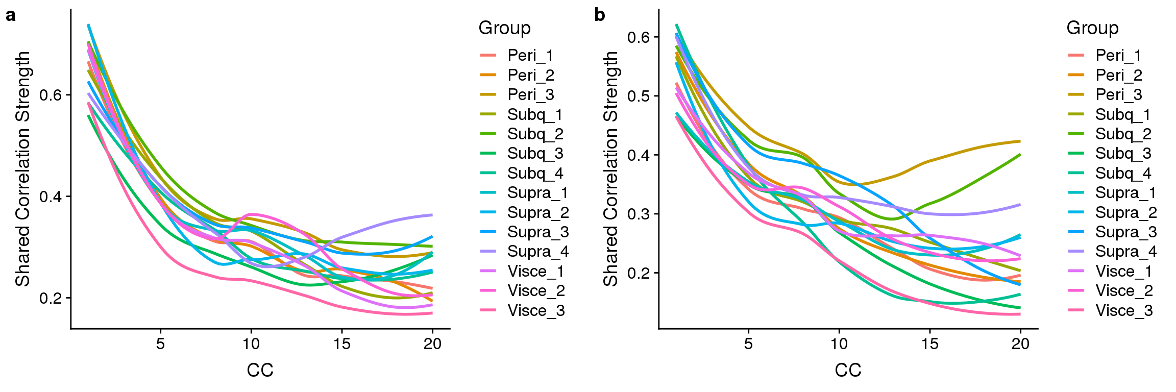
Expand here to see past versions of fig2-1.png:
| Version | Author | Date |
|---|---|---|
| eaa7e4a | PytrikFolkertsma | 2018-11-02 |
Discarded cells.
sfig2 <- plot_grid(
  p_discarded,
  p_discarded.ccregout,
  labels=c('a', 'b'),
  nrow=1
)
save_plot("plots/supplementary_figures/sfig_180504_alignment-discardedcells.pdf", sfig2, base_width=12, base_height=4)
sfig2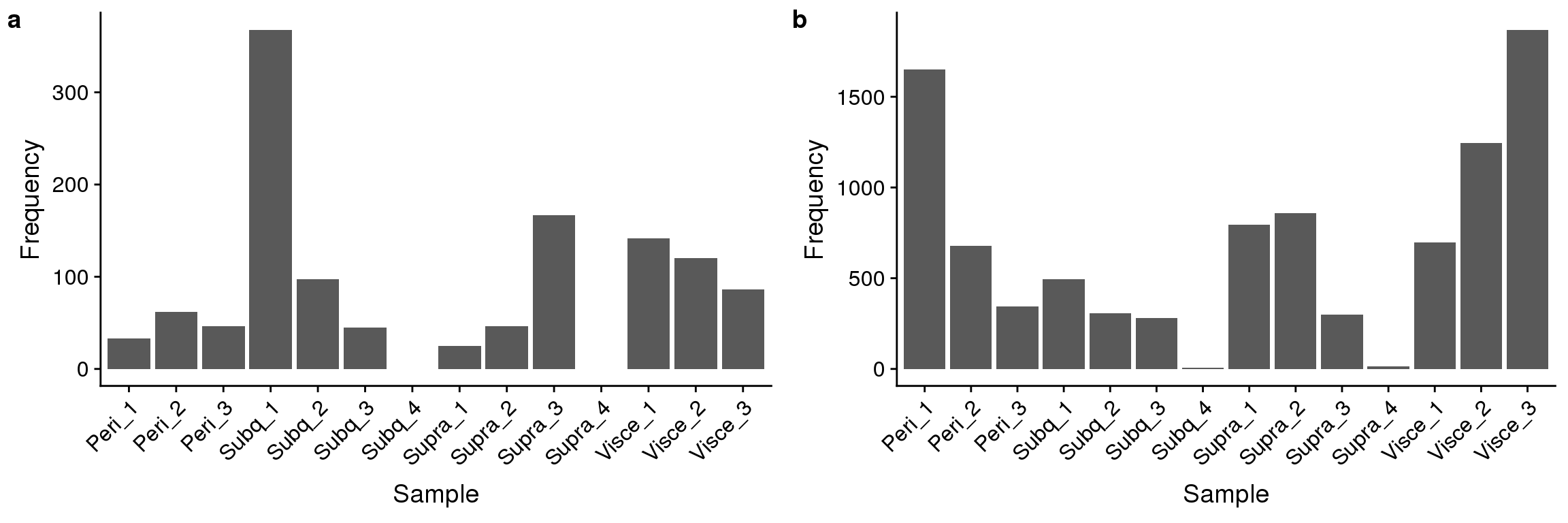
Expand here to see past versions of fi3-1.png:
| Version | Author | Date |
|---|---|---|
| eaa7e4a | PytrikFolkertsma | 2018-11-02 |
Session information
sessionInfo()R version 3.4.3 (2017-11-30)
Platform: x86_64-redhat-linux-gnu (64-bit)
Running under: Red Hat Enterprise Linux
Matrix products: default
BLAS/LAPACK: /usr/lib64/R/lib/libRblas.so
locale:
[1] LC_CTYPE=en_US.UTF-8 LC_NUMERIC=C
[3] LC_TIME=en_US.UTF-8 LC_COLLATE=en_US.UTF-8
[5] LC_MONETARY=en_US.UTF-8 LC_MESSAGES=en_US.UTF-8
[7] LC_PAPER=en_US.UTF-8 LC_NAME=C
[9] LC_ADDRESS=C LC_TELEPHONE=C
[11] LC_MEASUREMENT=en_US.UTF-8 LC_IDENTIFICATION=C
attached base packages:
[1] stats graphics grDevices utils datasets methods base
other attached packages:
[1] Seurat_2.3.4 Matrix_1.2-14 cowplot_0.9.3 ggplot2_3.0.0
loaded via a namespace (and not attached):
[1] Rtsne_0.13 colorspace_1.3-2 class_7.3-14
[4] modeltools_0.2-22 ggridges_0.5.0 mclust_5.4.1
[7] rprojroot_1.3-2 htmlTable_1.12 base64enc_0.1-3
[10] rstudioapi_0.7 proxy_0.4-22 flexmix_2.3-14
[13] bit64_0.9-7 mvtnorm_1.0-8 codetools_0.2-15
[16] splines_3.4.3 R.methodsS3_1.7.1 robustbase_0.93-2
[19] knitr_1.20 Formula_1.2-3 jsonlite_1.5
[22] workflowr_1.1.1 ica_1.0-2 cluster_2.0.7-1
[25] kernlab_0.9-27 png_0.1-7 R.oo_1.22.0
[28] compiler_3.4.3 httr_1.3.1 backports_1.1.2
[31] assertthat_0.2.0 lazyeval_0.2.1 lars_1.2
[34] acepack_1.4.1 htmltools_0.3.6 tools_3.4.3
[37] bindrcpp_0.2.2 igraph_1.2.2 gtable_0.2.0
[40] glue_1.3.0 RANN_2.6 reshape2_1.4.3
[43] dplyr_0.7.6 Rcpp_0.12.18 trimcluster_0.1-2.1
[46] gdata_2.18.0 ape_5.1 nlme_3.1-137
[49] iterators_1.0.10 fpc_2.1-11.1 gbRd_0.4-11
[52] lmtest_0.9-36 stringr_1.3.1 irlba_2.3.2
[55] gtools_3.8.1 DEoptimR_1.0-8 MASS_7.3-50
[58] zoo_1.8-3 scales_1.0.0 doSNOW_1.0.16
[61] parallel_3.4.3 RColorBrewer_1.1-2 yaml_2.2.0
[64] reticulate_1.10 pbapply_1.3-4 gridExtra_2.3
[67] rpart_4.1-13 segmented_0.5-3.0 latticeExtra_0.6-28
[70] stringi_1.2.4 foreach_1.4.4 checkmate_1.8.5
[73] caTools_1.17.1.1 bibtex_0.4.2 Rdpack_0.9-0
[76] SDMTools_1.1-221 rlang_0.2.2 pkgconfig_2.0.2
[79] dtw_1.20-1 prabclus_2.2-6 bitops_1.0-6
[82] evaluate_0.11 lattice_0.20-35 ROCR_1.0-7
[85] purrr_0.2.5 bindr_0.1.1 labeling_0.3
[88] htmlwidgets_1.2 bit_1.1-14 tidyselect_0.2.4
[91] plyr_1.8.4 magrittr_1.5 R6_2.2.2
[94] snow_0.4-2 gplots_3.0.1 Hmisc_4.1-1
[97] pillar_1.3.0 whisker_0.3-2 foreign_0.8-70
[100] withr_2.1.2 fitdistrplus_1.0-9 mixtools_1.1.0
[103] survival_2.42-6 nnet_7.3-12 tsne_0.1-3
[106] tibble_1.4.2 crayon_1.3.4 hdf5r_1.0.0
[109] KernSmooth_2.23-15 rmarkdown_1.10 grid_3.4.3
[112] data.table_1.11.4 git2r_0.23.0 metap_1.0
[115] digest_0.6.15 diptest_0.75-7 tidyr_0.8.1
[118] R.utils_2.7.0 stats4_3.4.3 munsell_0.5.0 This reproducible R Markdown analysis was created with workflowr 1.1.1