Last updated: 2018-11-07

workflowr checks: (Click a bullet for more information)

✔ R Markdown file: up-to-date

Great! Since the R Markdown file has been committed to the Git repository, you know the exact version of the code that produced these results.
✔ Environment: empty

Great job! The global environment was empty. Objects defined in the global environment can affect the analysis in your R Markdown file in unknown ways. For reproduciblity it’s best to always run the code in an empty environment.
✔ Seed: set.seed(20181026)

The command set.seed(20181026) was run prior to running the code in the R Markdown file. Setting a seed ensures that any results that rely on randomness, e.g. subsampling or permutations, are reproducible.
✔ Session information: recorded

Great job! Recording the operating system, R version, and package versions is critical for reproducibility.
✔ Repository version: 4db96e3
Great! You are using Git for version control. Tracking code development and connecting the code version to the results is critical for reproducibility. The version displayed above was the version of the Git repository at the time these results were generated.

Note that you need to be careful to ensure that all relevant files for the analysis have been committed to Git prior to generating the results (you can use wflow_publish or wflow_git_commit). workflowr only checks the R Markdown file, but you know if there are other scripts or data files that it depends on. Below is the status of the Git repository when the results were generated:
```
Ignored files:
    Ignored:    output/monocle/

Untracked files:
    Untracked:  plots/180504_monocle_noreg-ccreg.pdf
    Untracked:  plots/supplementary_figures/sfig_180504_monocle.pdf

Unstaged changes:
    Modified:   analysis/about.Rmd
    Modified:   analysis/index.Rmd
    Modified:   code/run-monocle.R
```
Note that any generated files, e.g. HTML, png, CSS, etc., are not included in this status report because it is ok for generated content to have uncommitted changes.

Expand here to see past versions:

File	Version	Author	Date	Message
Rmd	039a705	PytrikFolkertsma	2018-11-06	monocle

Notebook for Monocle trajectories of the 180504 dataset.

To investigate the robustness of the trajectories, the dataset was randomly downsampled on 1000 cells per sample. 4 different types of regressions were used when running the DDRTree algorithm.

library(Seurat)
library(monocle)

Loading all datasets.

cds.11 <- readRDS('output/monocle/180504/10x-180504-monocle-11')
cds.cc.11 <- readRDS('output/monocle/180504/10x-180504-monocle-cc-11')
cds.pm.umi.11 <- readRDS('output/monocle/180504/10x-180504-monocle-pm-umi-11')
cds.pm.umi.cc.11 <- readRDS('output/monocle/180504/10x-180504-monocle-pm-umi-cc-11')

cds.27 <- readRDS('output/monocle/180504/10x-180504-monocle-27')
cds.cc.27 <- readRDS('output/monocle/180504/10x-180504-monocle-cc-27')
cds.pm.umi.27 <- readRDS('output/monocle/180504/10x-180504-monocle-pm-umi-27')
cds.pm.umi.cc.27 <- readRDS('output/monocle/180504/10x-180504-monocle-pm-umi-cc-27')

cds.33 <- readRDS('output/monocle/180504/10x-180504-monocle-33')
cds.cc.33 <- readRDS('output/monocle/180504/10x-180504-monocle-cc-33')
cds.pm.umi.33 <- readRDS('output/monocle/180504/10x-180504-monocle-pm-umi-33')
cds.pm.umi.cc.33 <- readRDS('output/monocle/180504/10x-180504-monocle-pm-umi-cc-33')

cds.53 <- readRDS('output/monocle/180504/10x-180504-monocle-53')
cds.cc.53 <- readRDS('output/monocle/180504/10x-180504-monocle-cc-53')
cds.pm.umi.53 <- readRDS('output/monocle/180504/10x-180504-monocle-pm-umi-53')
cds.pm.umi.cc.53 <- readRDS('output/monocle/180504/10x-180504-monocle-pm-umi-cc-53')

Trajectories of one subset

Trajectories of one subset, coloured by sample and cell cycle phase. Topleft: no regression. Topright: cell cycle regression. Bottom left: percent.mito + nUMI regression. Bottom right: percent.mito + nUMI + cell cycle regression.

plot_grid(
  plot_cell_trajectory(cds.11, color_by='depot'),
  plot_cell_trajectory(cds.cc.11, color_by='depot'),
  plot_cell_trajectory(cds.pm.umi.11, color_by='depot'),
  plot_cell_trajectory(cds.pm.umi.cc.11, color_by='depot'),
  nrow=2)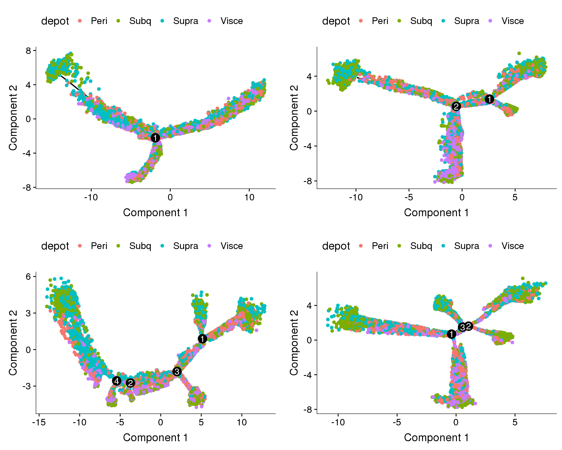

plot_grid(
  plot_cell_trajectory(cds.11, color_by='Phase'),
  plot_cell_trajectory(cds.cc.11, color_by='Phase'),
  plot_cell_trajectory(cds.pm.umi.11, color_by='Phase'),
  plot_cell_trajectory(cds.pm.umi.cc.11, color_by='Phase'),
  nrow=2)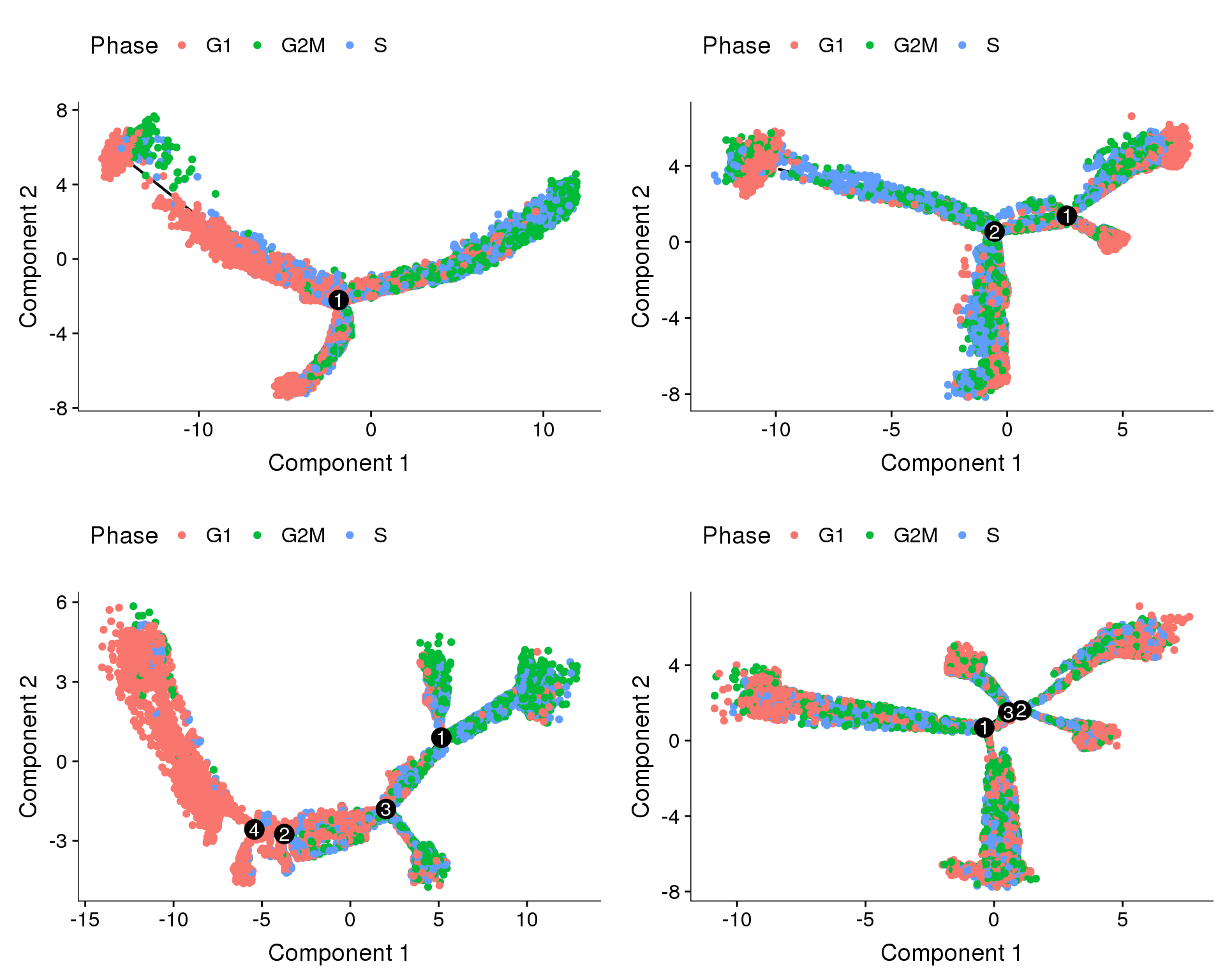

Trajectories, no regression

Trajectories of the 4 subsets with no variables regressed out. The ordering of the cells seems to be influenced by the cell cycle state (though not completely). Interestingly in three of the trajectories there is a branch split.

plot_grid(
  plot_cell_trajectory(cds.11, color_by='Phase'),
  plot_cell_trajectory(cds.27, color_by='Phase'),
  plot_cell_trajectory(cds.33, color_by='Phase'),
  plot_cell_trajectory(cds.53, color_by='Phase'),
  nrow=2)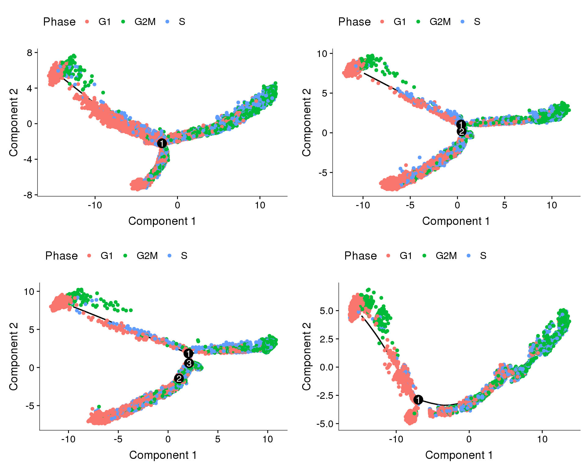

Does the branch split discriminate between depots?

plot_grid(
  plot_cell_trajectory(cds.11, color_by='depot'),
  plot_cell_trajectory(cds.27, color_by='depot'),
  plot_cell_trajectory(cds.33, color_by='depot'),
  plot_cell_trajectory(cds.53, color_by='depot'),
  nrow=2)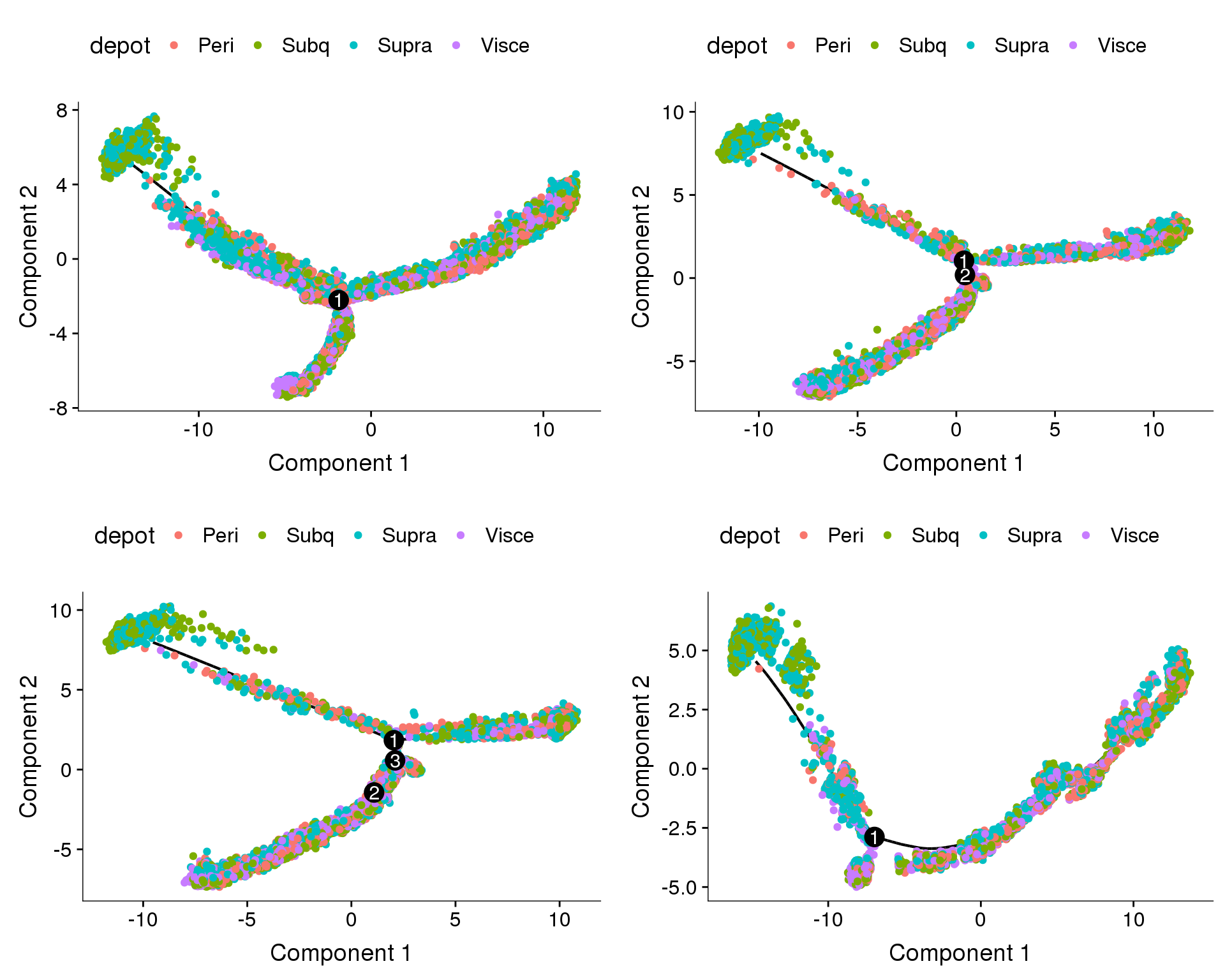

Trajectories, cell cycle regression

Trajectories of the 4 subsets with cell cycle effects regressed out. Topleft, bottom left and bottom right look similar but all have different number of branching points.

plot_grid(
  plot_cell_trajectory(cds.cc.11, color_by='Phase'),
  plot_cell_trajectory(cds.cc.27, color_by='Phase'),
  plot_cell_trajectory(cds.cc.33, color_by='Phase'),
  plot_cell_trajectory(cds.cc.53, color_by='Phase'),
  nrow=2)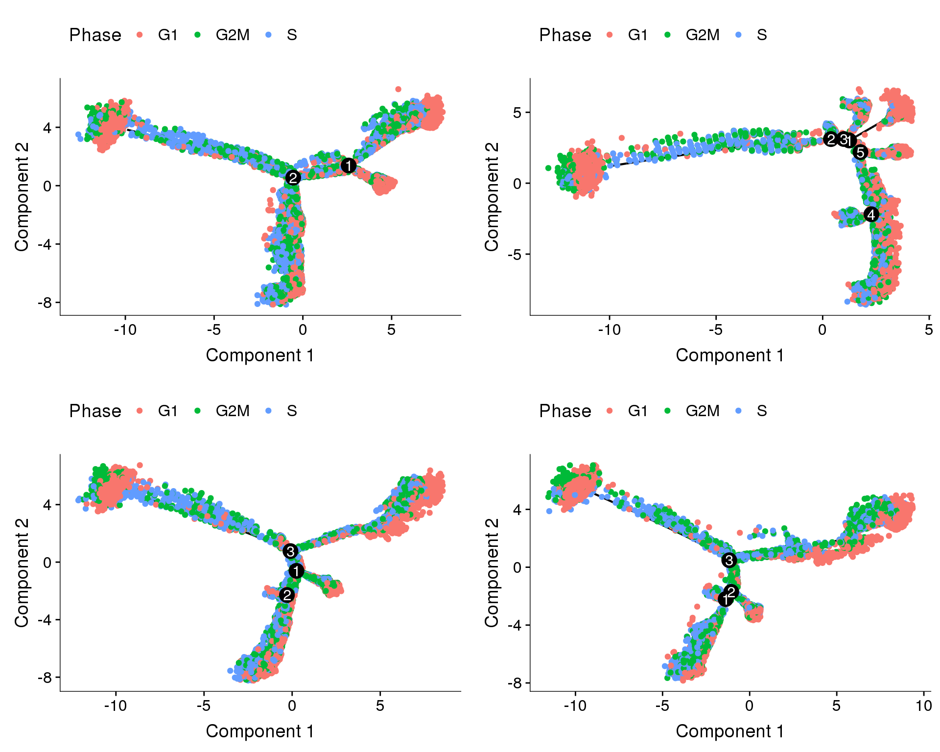

Coloured on depot. Branches do not

plot_grid(
  plot_cell_trajectory(cds.cc.11, color_by='depot'),
  plot_cell_trajectory(cds.cc.27, color_by='depot'),
  plot_cell_trajectory(cds.cc.33, color_by='depot'),
  plot_cell_trajectory(cds.cc.53, color_by='depot'),
  nrow=2)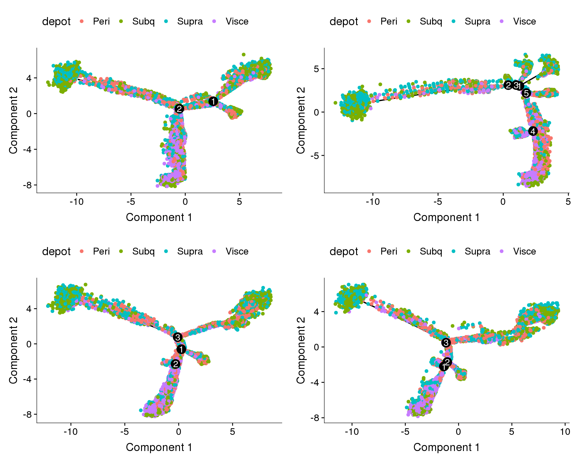

Trajectories, percent.mito + nUMI regression

In general all cells seem to follow one direction, and the general shape of the trajectories are similar. The branch splits in the trajectories above (no regression and cell cycle regression) could be the effects of differences in percent.mito and nUMI, and that’s why we don’t see that here.

plot_grid(
  plot_cell_trajectory(cds.pm.umi.11, color_by='Phase'),
  plot_cell_trajectory(cds.pm.umi.27, color_by='Phase'),
  plot_cell_trajectory(cds.pm.umi.33, color_by='Phase'),
  plot_cell_trajectory(cds.pm.umi.53, color_by='Phase'),
  nrow=2)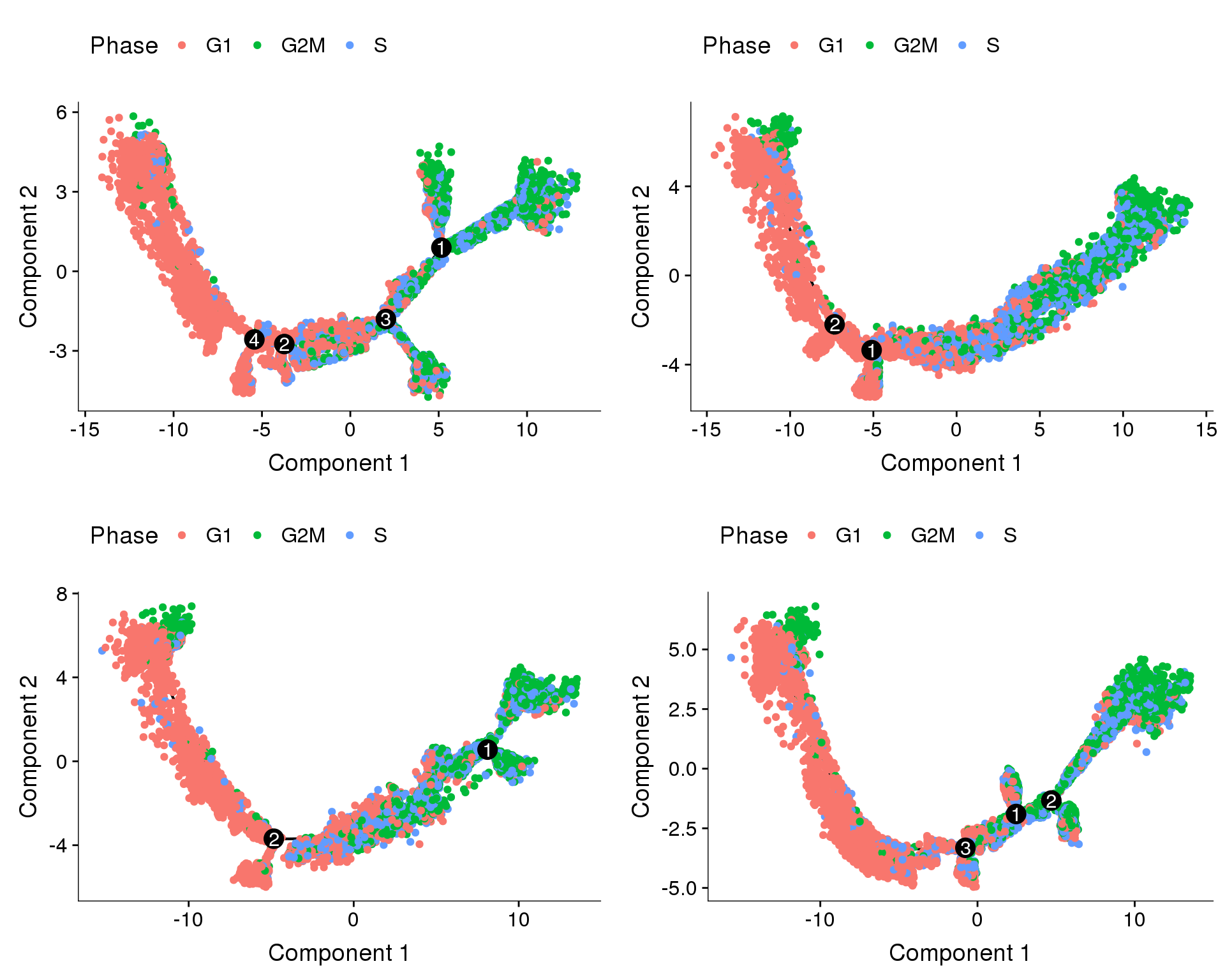

Trajectories, percent.mito + nUMI + cell cycle regression

Trajectories with percent.mito, nUMI and cell cycle effects regressed out. Doesn’t look very convincing.

plot_grid(
  plot_cell_trajectory(cds.pm.umi.cc.11, color_by='depot'),
  plot_cell_trajectory(cds.pm.umi.cc.27, color_by='depot'),
  plot_cell_trajectory(cds.pm.umi.cc.33, color_by='depot'),
  plot_cell_trajectory(cds.pm.umi.cc.53, color_by='depot'),
  nrow=2)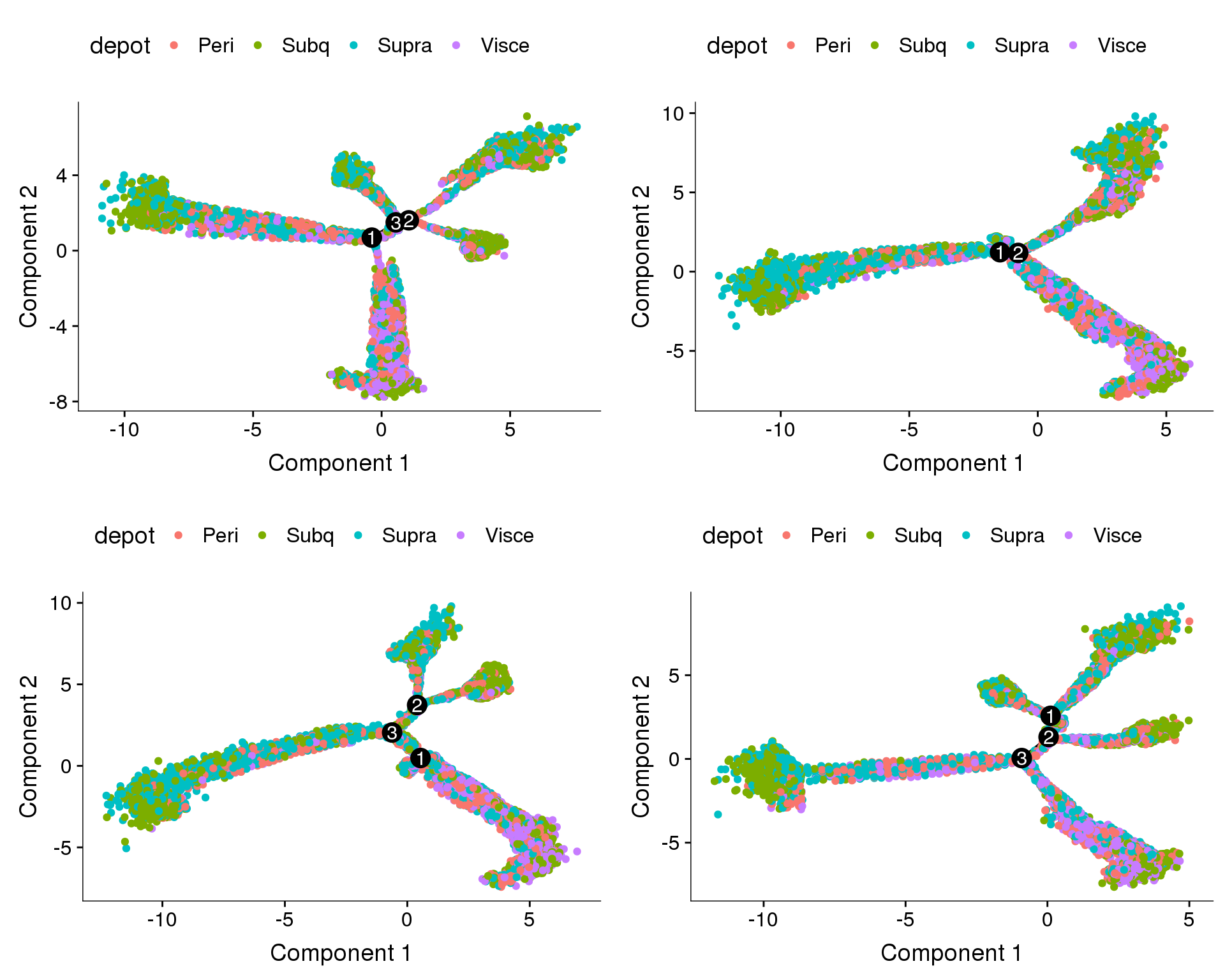

Figures for report

a = trajectory without regressions, coloured on cell cycle phase. b = trajectory with cell cycle effects regressed out, coloured on depot.

fig <- plot_grid(
  plot_cell_trajectory(cds.11, color_by='Phase'),
  plot_cell_trajectory(cds.cc.11, color_by='depot'),
  nrow=1, labels='auto')
save_plot("plots/180504_monocle_noreg-ccreg.pdf", fig, base_width=12, base_height=5)
fig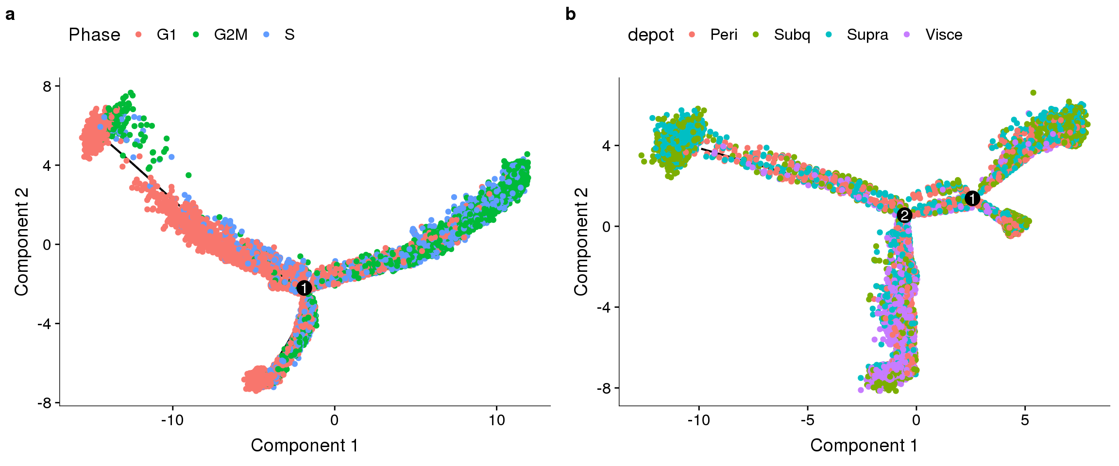

Supplementary figures

noreg <- plot_grid(
  plot_cell_trajectory(cds.11, color_by='Phase', cell_size = 0.5),
  plot_cell_trajectory(cds.27, color_by='Phase', cell_size = 0.5),
  plot_cell_trajectory(cds.33, color_by='Phase', cell_size = 0.5),
  plot_cell_trajectory(cds.53, color_by='Phase', cell_size = 0.5),
  nrow=1)

ccreg <- plot_grid(
  plot_cell_trajectory(cds.cc.11, color_by='Phase', cell_size = 0.5),
  plot_cell_trajectory(cds.cc.27, color_by='Phase', cell_size = 0.5),
  plot_cell_trajectory(cds.cc.33, color_by='Phase', cell_size = 0.5),
  plot_cell_trajectory(cds.cc.53, color_by='Phase', cell_size = 0.5),
  nrow=1)

pmumireg <- plot_grid(
  plot_cell_trajectory(cds.pm.umi.11, color_by='Phase', cell_size = 0.5),
  plot_cell_trajectory(cds.pm.umi.27, color_by='Phase', cell_size = 0.5),
  plot_cell_trajectory(cds.pm.umi.33, color_by='Phase', cell_size = 0.5),
  plot_cell_trajectory(cds.pm.umi.53, color_by='Phase', cell_size = 0.5),
  nrow=1)

pmumiccreg <- plot_grid(
  plot_cell_trajectory(cds.pm.umi.cc.11, color_by='Phase', cell_size = 0.5),
  plot_cell_trajectory(cds.pm.umi.cc.27, color_by='Phase', cell_size = 0.5),
  plot_cell_trajectory(cds.pm.umi.cc.33, color_by='Phase', cell_size = 0.5),
  plot_cell_trajectory(cds.pm.umi.cc.53, color_by='Phase', cell_size = 0.5),
  nrow=1)

sfig <- plot_grid(
  noreg,
  ccreg,
  pmumireg,
  pmumiccreg,
  labels='auto', nrow=4
)

save_plot("plots/supplementary_figures/sfig_180504_monocle.pdf", sfig, base_width=12, base_height=12)
sfig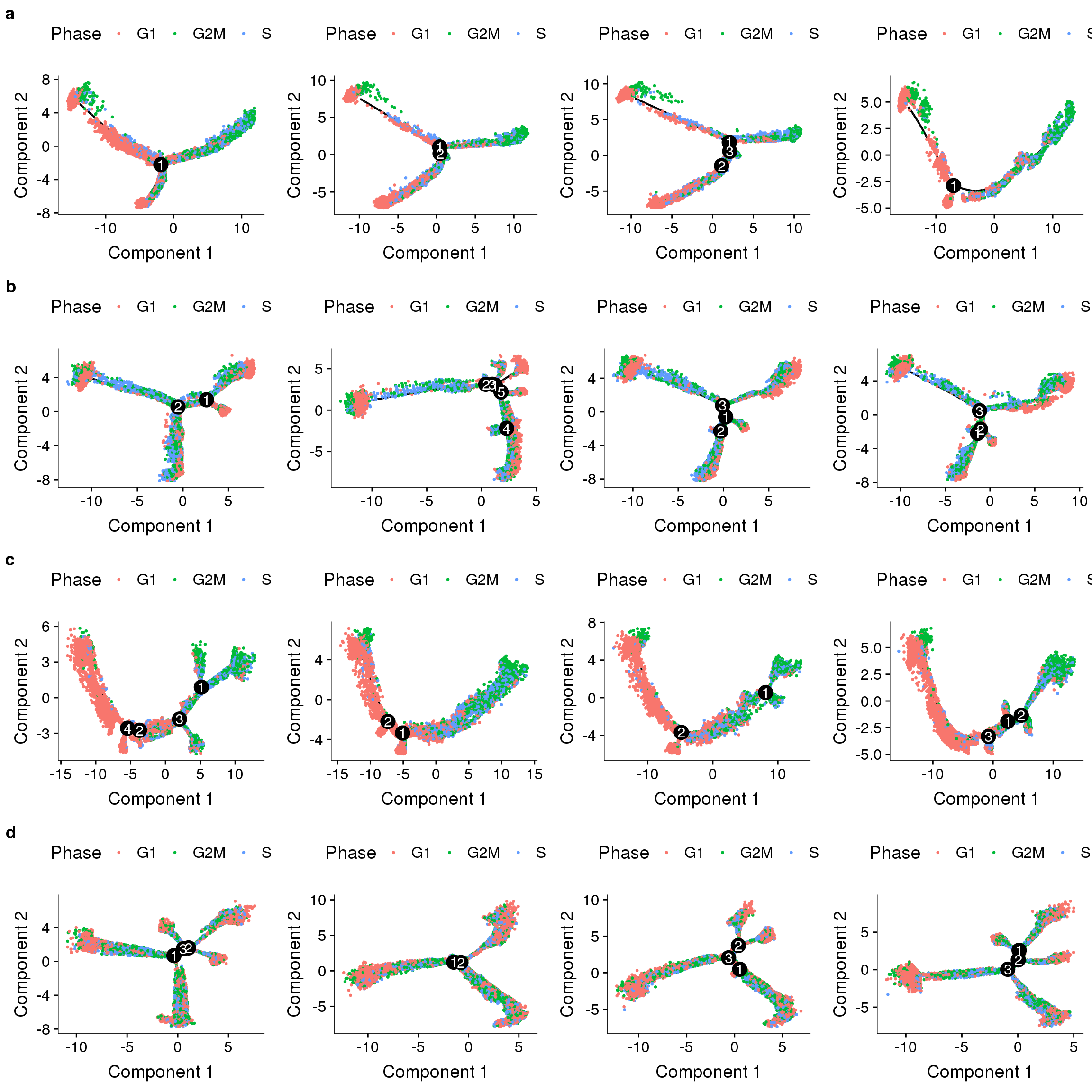

Session information

sessionInfo()

R version 3.4.3 (2017-11-30)
Platform: x86_64-redhat-linux-gnu (64-bit)
Running under: Red Hat Enterprise Linux

Matrix products: default
BLAS/LAPACK: /usr/lib64/R/lib/libRblas.so

locale:
 [1] LC_CTYPE=en_US.UTF-8       LC_NUMERIC=C              
 [3] LC_TIME=en_US.UTF-8        LC_COLLATE=en_US.UTF-8    
 [5] LC_MONETARY=en_US.UTF-8    LC_MESSAGES=en_US.UTF-8   
 [7] LC_PAPER=en_US.UTF-8       LC_NAME=C                 
 [9] LC_ADDRESS=C               LC_TELEPHONE=C            
[11] LC_MEASUREMENT=en_US.UTF-8 LC_IDENTIFICATION=C       

attached base packages:
 [1] splines   stats4    parallel  stats     graphics  grDevices utils    
 [8] datasets  methods   base     

other attached packages:
 [1] monocle_2.6.4       DDRTree_0.1.5       irlba_2.3.2        
 [4] VGAM_1.0-6          Biobase_2.38.0      BiocGenerics_0.24.0
 [7] Seurat_2.3.4        Matrix_1.2-14       cowplot_0.9.3      
[10] ggplot2_3.0.0      

loaded via a namespace (and not attached):
  [1] Rtsne_0.13             colorspace_1.3-2       class_7.3-14          
  [4] modeltools_0.2-22      ggridges_0.5.0         mclust_5.4.1          
  [7] rprojroot_1.3-2        htmlTable_1.12         base64enc_0.1-3       
 [10] rstudioapi_0.7         proxy_0.4-22           ggrepel_0.8.0         
 [13] flexmix_2.3-14         bit64_0.9-7            mvtnorm_1.0-8         
 [16] codetools_0.2-15       R.methodsS3_1.7.1      docopt_0.6            
 [19] robustbase_0.93-2      knitr_1.20             Formula_1.2-3         
 [22] jsonlite_1.5           workflowr_1.1.1        ica_1.0-2             
 [25] cluster_2.0.7-1        kernlab_0.9-27         png_0.1-7             
 [28] R.oo_1.22.0            pheatmap_1.0.10        compiler_3.4.3        
 [31] httr_1.3.1             backports_1.1.2        assertthat_0.2.0      
 [34] lazyeval_0.2.1         limma_3.34.9           lars_1.2              
 [37] acepack_1.4.1          htmltools_0.3.6        tools_3.4.3           
 [40] bindrcpp_0.2.2         igraph_1.2.2           gtable_0.2.0          
 [43] glue_1.3.0             RANN_2.6               reshape2_1.4.3        
 [46] dplyr_0.7.6            Rcpp_0.12.18           slam_0.1-43           
 [49] trimcluster_0.1-2.1    gdata_2.18.0           ape_5.1               
 [52] nlme_3.1-137           iterators_1.0.10       fpc_2.1-11.1          
 [55] gbRd_0.4-11            lmtest_0.9-36          stringr_1.3.1         
 [58] gtools_3.8.1           DEoptimR_1.0-8         MASS_7.3-50           
 [61] zoo_1.8-3              scales_1.0.0           doSNOW_1.0.16         
 [64] RColorBrewer_1.1-2     yaml_2.2.0             reticulate_1.10       
 [67] pbapply_1.3-4          gridExtra_2.3          rpart_4.1-13          
 [70] segmented_0.5-3.0      fastICA_1.2-1          latticeExtra_0.6-28   
 [73] stringi_1.2.4          foreach_1.4.4          checkmate_1.8.5       
 [76] caTools_1.17.1.1       densityClust_0.3       bibtex_0.4.2          
 [79] matrixStats_0.54.0     Rdpack_0.9-0           SDMTools_1.1-221      
 [82] rlang_0.2.2            pkgconfig_2.0.2        dtw_1.20-1            
 [85] prabclus_2.2-6         bitops_1.0-6           qlcMatrix_0.9.7       
 [88] evaluate_0.11          lattice_0.20-35        ROCR_1.0-7            
 [91] purrr_0.2.5            bindr_0.1.1            labeling_0.3          
 [94] htmlwidgets_1.2        bit_1.1-14             tidyselect_0.2.4      
 [97] plyr_1.8.4             magrittr_1.5           R6_2.2.2              
[100] snow_0.4-2             gplots_3.0.1           Hmisc_4.1-1           
[103] combinat_0.0-8         pillar_1.3.0           whisker_0.3-2         
[106] foreign_0.8-71         withr_2.1.2            fitdistrplus_1.0-9    
[109] mixtools_1.1.0         survival_2.42-6        nnet_7.3-12           
[112] tsne_0.1-3             tibble_1.4.2           crayon_1.3.4          
[115] hdf5r_1.0.0            KernSmooth_2.23-15     rmarkdown_1.10        
[118] viridis_0.5.1          grid_3.4.3             data.table_1.11.4     
[121] FNN_1.1.2.1            git2r_0.23.0           sparsesvd_0.1-4       
[124] HSMMSingleCell_0.112.0 metap_1.0              digest_0.6.16         
[127] diptest_0.75-7         tidyr_0.8.1            R.utils_2.7.0         
[130] munsell_0.5.0          viridisLite_0.3.0

This reproducible R Markdown analysis was created with workflowr 1.1.1