Introduction

# Library

library(edgeR)

Loading required package: limma

library(limma)
library(VennDiagram)

Warning: package 'VennDiagram' was built under R version 3.4.4

Loading required package: grid

Loading required package: futile.logger

library(cowplot)

Warning: package 'cowplot' was built under R version 3.4.4

Loading required package: ggplot2

Warning: package 'ggplot2' was built under R version 3.4.4

Attaching package: 'cowplot'

The following object is masked from 'package:ggplot2':

    ggsave

# Read in the data

tx.salmon <- readRDS("../data/counts_hg38_gc_txsalmon.RData")
salmon_counts<- as.data.frame(tx.salmon$counts)


#tx.salmon <- readRDS("../data/counts_hg38_gc_dds.RData")
#salmon_counts<- as.data.frame(tx.salmon)


# Subset to T1-T3

salmon_counts <- salmon_counts[,1:144]

# Read in the clinical covariates

clinical_sample_info <- read.csv("../data/lm_covar_fixed_random.csv")
dim(clinical_sample_info)

[1] 156  13

# Subset to T1-T3

clinical_sample <- clinical_sample_info[1:144,(-12)]

dim(clinical_sample)

[1] 144  12

Differential expression pipeline

# Filter lowly expressed reads

cpm <- cpm(salmon_counts, log=TRUE)

expr_cutoff <- 1.5
hist(cpm, main = "log2(CPM) values in unfiltered data", breaks = 100, xlab = "log2(CPM) values")
abline(v = expr_cutoff, col = "red", lwd = 3)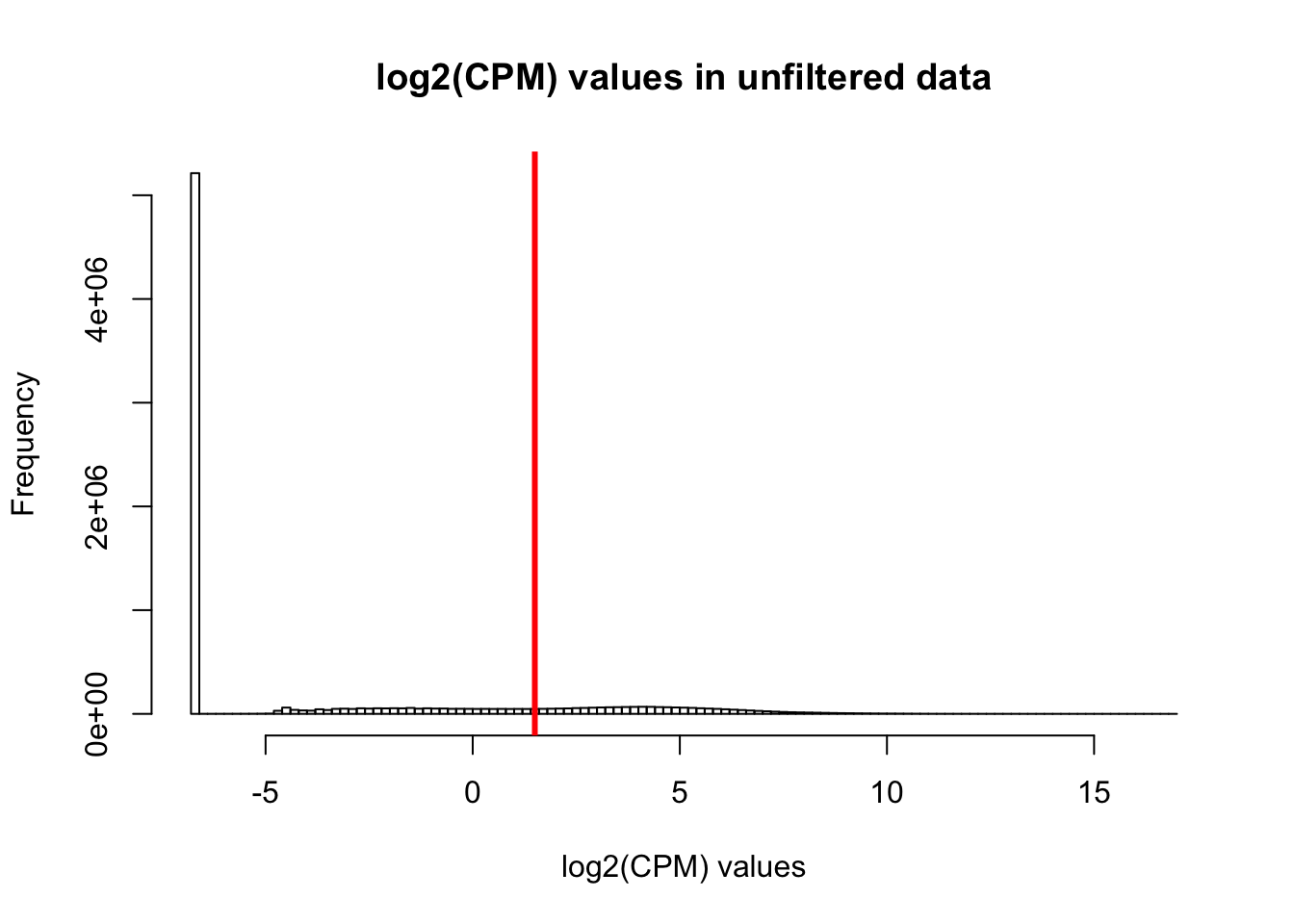

hist(cpm, main = "log2(CPM) values in unfiltered data", breaks = 100, xlab = "log2(CPM) values", ylim = c(0, 100000))
abline(v = expr_cutoff, col = "red", lwd = 3)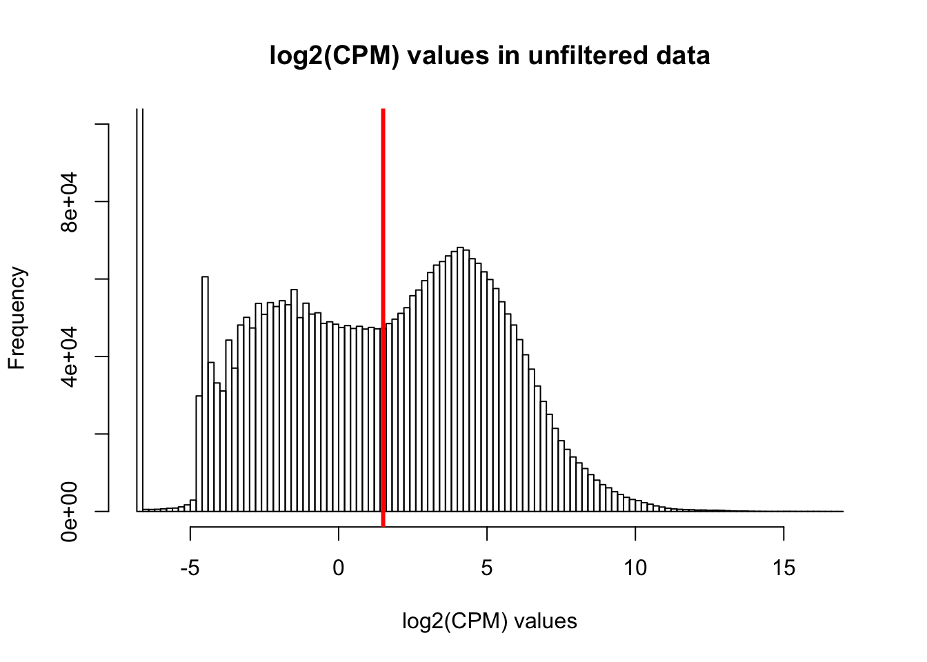

# Basic filtering
cpm_filtered <- (rowSums(cpm > 1.5) > 72)

genes_in_cutoff <- cpm[cpm_filtered==TRUE,]

hist(as.numeric(unlist(genes_in_cutoff)), main = "log2(CPM) values in filtered data", breaks = 100, xlab = "log2(CPM) values")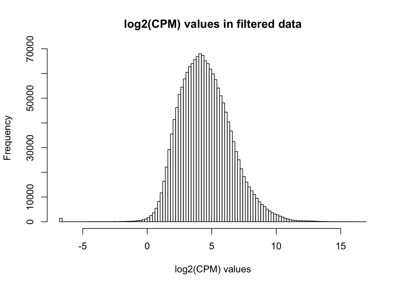

# Find the original counts of all of the genes that fit the criteria 

counts_genes_in_cutoff <- salmon_counts[cpm_filtered==TRUE,]
dim(counts_genes_in_cutoff)

[1] 11619   144

# Filter out hemoglobin

counts_genes_in_cutoff <-  counts_genes_in_cutoff[which( rownames(counts_genes_in_cutoff) != "HBB" ),]
counts_genes_in_cutoff <-  counts_genes_in_cutoff[which( rownames(counts_genes_in_cutoff) != "HBA2" ),]
counts_genes_in_cutoff <-  counts_genes_in_cutoff[which( rownames(counts_genes_in_cutoff) != "HBA1" ),]

# Take the TMM of the counts only for the genes that remain after filtering

dge_in_cutoff <- DGEList(counts=as.matrix(counts_genes_in_cutoff), genes=rownames(counts_genes_in_cutoff), group = as.character(t(clinical_sample$Individual)))
dge_in_cutoff <- calcNormFactors(dge_in_cutoff)

cpm_in_cutoff <- cpm(dge_in_cutoff, normalized.lib.sizes=TRUE, log=TRUE)

pca_genes <- prcomp(t(cpm_in_cutoff), scale = T, retx = TRUE, center = TRUE)

matrixpca <- pca_genes$x
PC1 <- matrixpca[,1]
PC2 <- matrixpca[,2]
pc3 <- matrixpca[,3]
pc4 <- matrixpca[,4]
pc5 <- matrixpca[,5]

pcs <- data.frame(PC1, PC2, pc3, pc4, pc5)

summary <- summary(pca_genes)

head(summary$importance[2,1:5])

    PC1     PC2     PC3     PC4     PC5 
0.25012 0.13000 0.08757 0.05524 0.03285 

norm_count <- ggplot(data=pcs, aes(x=PC1, y=PC2, color= as.factor(clinical_sample$Time))) + geom_point(aes(colour = as.factor(clinical_sample$Time))) + ggtitle("PCA of normalized counts") + scale_color_discrete(name = "Time")

plot_grid(norm_count)

clinical_sample[,1] <- as.factor(clinical_sample[,1])

clinical_sample[,2] <- as.factor(clinical_sample[,2])

clinical_sample[,4] <- as.factor(clinical_sample[,4])

clinical_sample[,5] <- as.factor(clinical_sample[,5])

clinical_sample[,6] <- as.factor(clinical_sample[,6])


# Create the design matrix

# Use the standard treatment-contrasts parametrization. See Ch. 9 of limma
# User's Guide.

design <- model.matrix(~as.factor(Time) + Age + as.factor(Race) + as.factor(BE_GROUP) + as.factor(psychmeds) + RBC + AN + AE + AL  + RIN + Change_weight, data = clinical_sample)
colnames(design) <- c("Intercept", "Time2", "Time3", "Race3", "Race5", "Age", "BE", "Psychmeds", "RBC", "AN", "AE", "AL", "RIN", "Change_weight")


# Fit model 

# Model individual as a random effect.
# Recommended to run both voom and duplicateCorrelation twice.
# https://support.bioconductor.org/p/59700/#67620

cpm.voom <- voom(dge_in_cutoff, design, normalize.method="none")
#check_rel <- duplicateCorrelation(cpm.voom, design, block = clinical_sample$Individual)
check_rel_correlation <-  0.1179835
cpm.voom.corfit <- voom(dge_in_cutoff, design, normalize.method="none", plot = TRUE, block = clinical_sample$Individual, correlation = check_rel_correlation)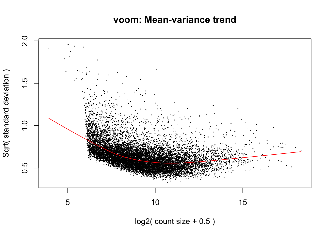

#check_rel <- duplicateCorrelation(cpm.voom.corfit, design, block = clinical_sample$Individual)
check_rel_correlation <- 0.1188083

plotDensities(cpm.voom.corfit[,1])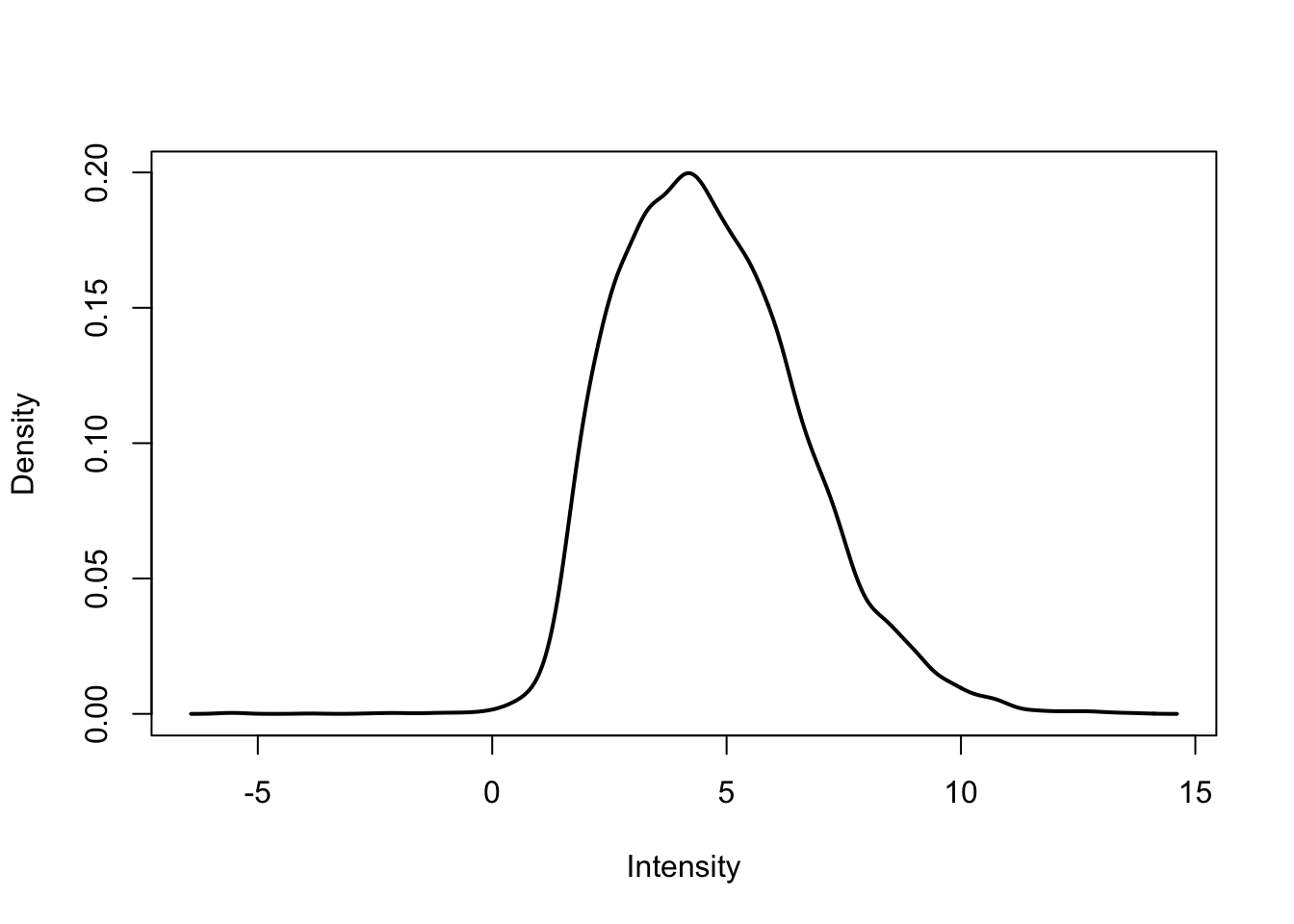

plotDensities(cpm.voom.corfit[,2])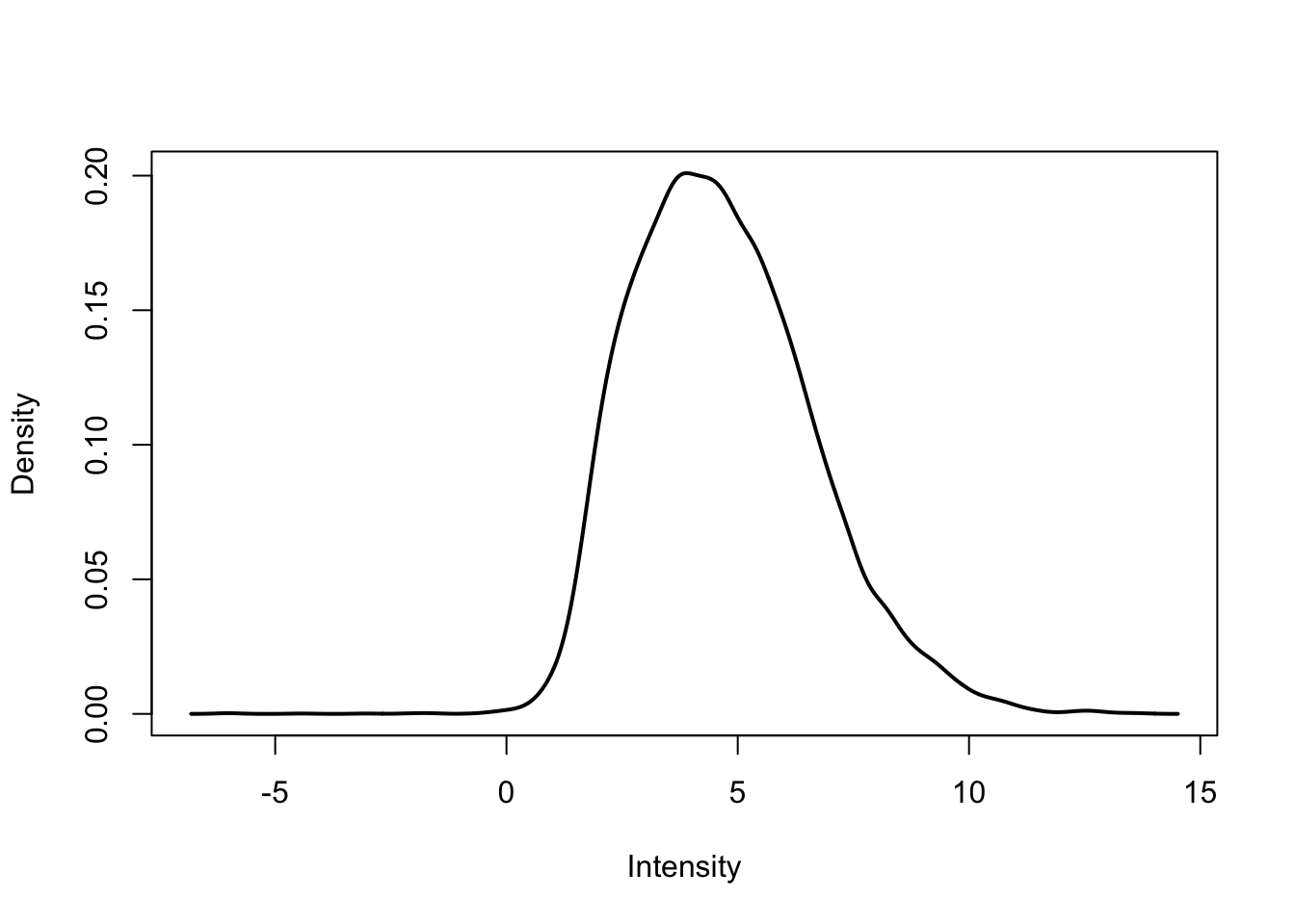

plotDensities(cpm.voom.corfit[,3])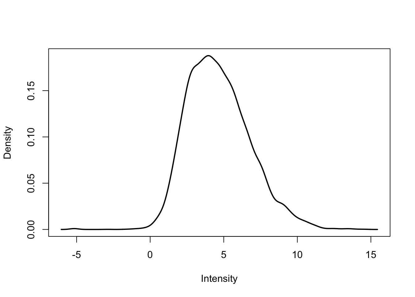

pca_genes <- prcomp(t(cpm.voom.corfit$E), scale = T, retx = TRUE, center = TRUE)

matrixpca <- pca_genes$x
PC1 <- matrixpca[,1]
PC2 <- matrixpca[,2]
pc3 <- matrixpca[,3]
pc4 <- matrixpca[,4]
pc5 <- matrixpca[,5]

pcs <- data.frame(PC1, PC2, pc3, pc4, pc5)

summary <- summary(pca_genes)

head(summary$importance[2,1:5])

    PC1     PC2     PC3     PC4     PC5 
0.25066 0.13028 0.08774 0.05501 0.03289 

ggplot(data=pcs, aes(x=PC1, y=PC2, color=clinical_sample$Time)) + geom_point(aes(colour = as.factor(clinical_sample$Time))) + ggtitle("PCA of normalized counts") + scale_color_discrete(name = "Time")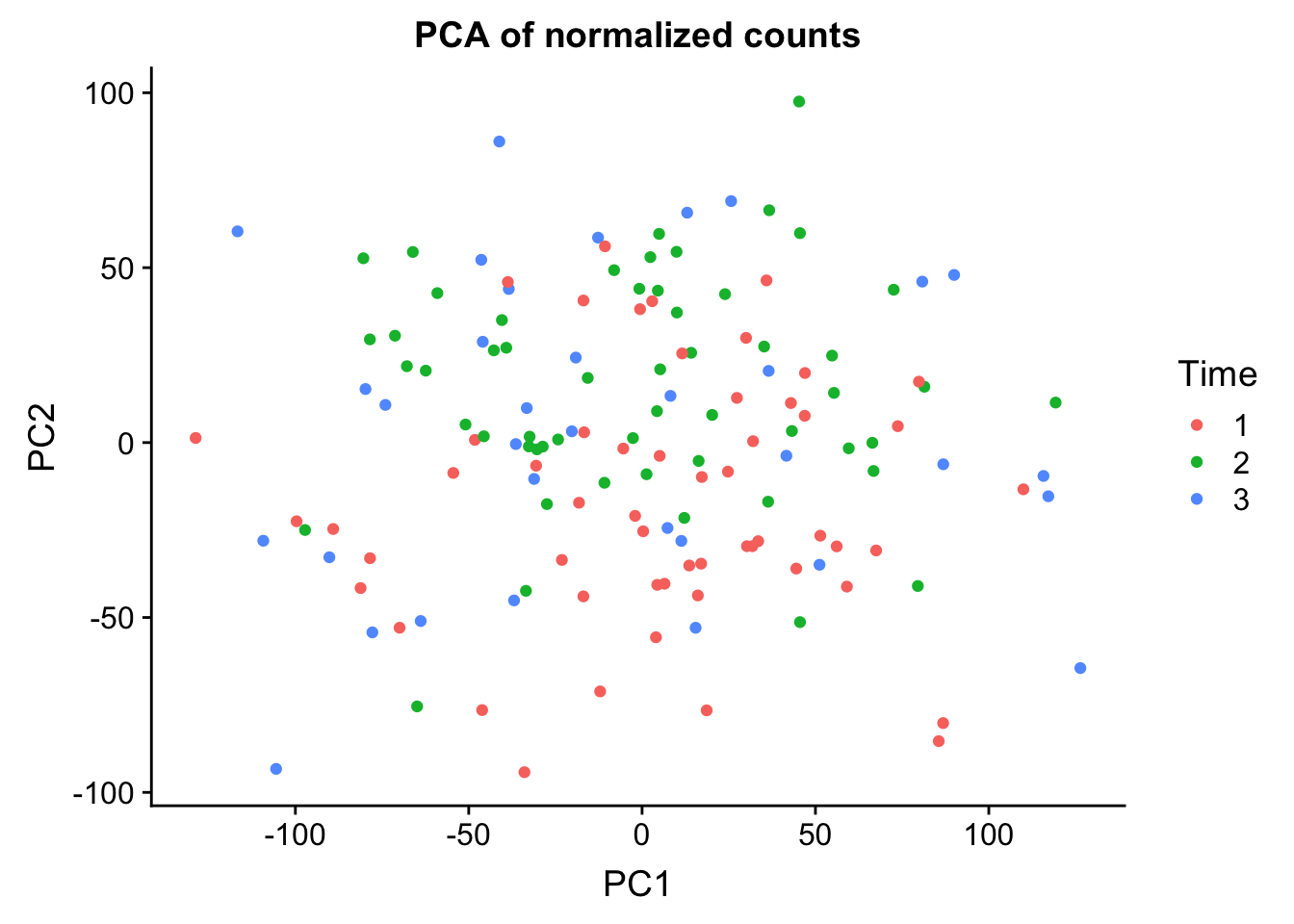

# Run lmFit and eBayes in limma

fit <- lmFit(cpm.voom.corfit, design, block=clinical_sample$Individual, correlation=check_rel_correlation)

# In the contrast matrix, have the time points

cm1 <- makeContrasts(Time1v2 = Time2, Time2v3 = Time3 - Time2, levels = design)

#cm1 <- makeContrasts(Time1v2 = Time2, Time2v3 = Time3, levels = design)

# Fit the new model
diff_species <- contrasts.fit(fit, cm1)
fit1 <- eBayes(diff_species)

FDR_level <- 0.05

Time1v2 =topTable(fit1, coef=1, adjust="BH", number=Inf, sort.by="none")
Time2v3 =topTable(fit1, coef=2, adjust="BH", number=Inf, sort.by="none")

#plot(fit1$coefficients[,1], fit1$coefficients[,2])
plot(Time1v2$logFC, Time2v3$logFC)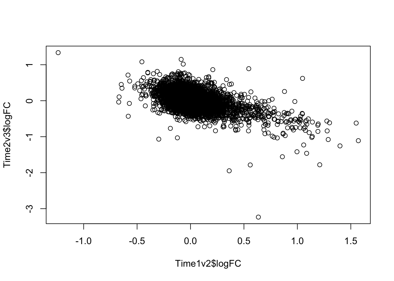

plot(Time1v2$t, Time2v3$t)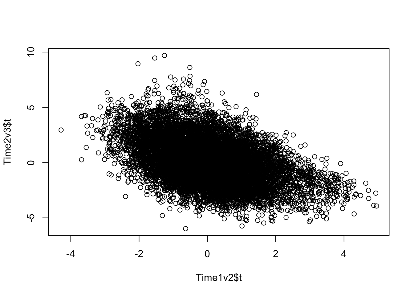

plot(Time1v2$adj.P.Val, Time2v3$adj.P.Val)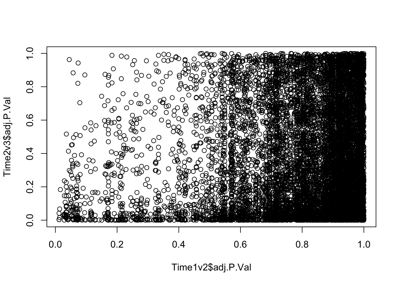

dim(Time1v2[which(Time1v2$adj.P.Val < FDR_level),])

[1] 44  7

dim(Time2v3[which(Time2v3$adj.P.Val < FDR_level),])

[1] 1991    7

head(topTable(fit1, coef=1, adjust="BH", number=100, sort.by="T"))

          genes     logFC   AveExpr        t      P.Value  adj.P.Val
ABALON   ABALON 1.2887511  2.170769 4.952850 2.150985e-06 0.01180735
CTNNAL1 CTNNAL1 1.1912596  1.961155 4.930330 2.371899e-06 0.01180735
DCAF6     DCAF6 0.5014972  5.448487 4.872156 3.049420e-06 0.01180735
RNF10     RNF10 0.8199629  8.824150 4.724856 5.712588e-06 0.01374242
GPR146   GPR146 1.1950100  4.684580 4.716587 5.915299e-06 0.01374242
ALAS2     ALAS2 1.5503665 10.196972 4.636501 8.275050e-06 0.01602050
               B
ABALON  3.830754
CTNNAL1 3.499233
DCAF6   4.297388
RNF10   3.704913
GPR146  3.664174
ALAS2   3.323802

head(topTable(fit1, coef=2, adjust="BH", number=100, sort.by="T"))

                    genes     logFC  AveExpr        t      P.Value
MPHOSPH8         MPHOSPH8 0.7313353 6.149241 9.694977 3.460385e-17
CYP20A1           CYP20A1 0.6466663 4.471779 9.464323 1.306430e-16
DFFA                 DFFA 0.5483855 4.550302 8.948600 2.491086e-15
RTF1                 RTF1 0.5960518 5.568985 8.607535 1.714095e-14
RP11-83A24.2 RP11-83A24.2 1.0179575 2.905414 7.815085 1.392854e-12
CTA-292E10.9 CTA-292E10.9 0.8056242 3.931612 7.747620 2.012435e-12
                adj.P.Val        B
MPHOSPH8     4.019583e-13 28.39307
CYP20A1      7.587744e-13 26.98074
DFFA         9.645486e-12 24.18296
RTF1         4.977732e-11 22.41650
RP11-83A24.2 3.235878e-09 17.81809
CTA-292E10.9 3.896074e-09 17.73477

Make a Venn Diagram of the DE genes

# FDR 1%
FDR_level <- 0.01

Time12 <- rownames(Time1v2[which(Time1v2$adj.P.Val < FDR_level),])

Time23 <- rownames(Time2v3[which(Time2v3$adj.P.Val < FDR_level),])

mylist <- list()
mylist[["DE T1 to T2"]] <- Time12
mylist[["DE T2 to T3"]] <- Time23

# Make as pdf 
Four_comp <- venn.diagram(mylist, filename= NULL, main="DE genes between timepoints (1% FDR)", cex=1.5 , fill = NULL, lty=1, height=2000, width=2000, rotation.degree = 180, scaled = FALSE, cat.pos = c(0,0))

grid.draw(Four_comp)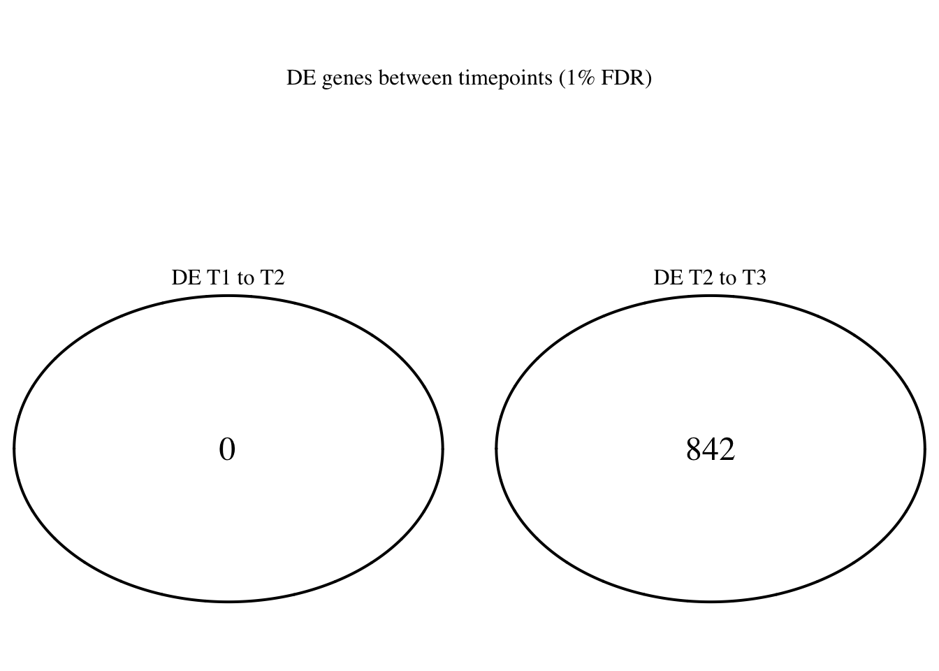

dev.off()

null device 
          1 

#pdf(file = "~/Dropbox/Figures/DET1_T2_change_weight_FDR1.pdf")
#  grid.draw(Four_comp)
#dev.off()

# FDR 5%

FDR_level <- 0.05
Time12 <- rownames(Time1v2[which(Time1v2$adj.P.Val < FDR_level),])

Time23 <- rownames(Time2v3[which(Time2v3$adj.P.Val < FDR_level),])

mylist <- list()
mylist[["DE T1 to T2"]] <- Time12
mylist[["DE T2 to T3"]] <- Time23

# Make as pdf 
Four_comp <- venn.diagram(mylist, filename= NULL, main="DE genes between timepoints (5% FDR)", cex=1.5 , fill = NULL, lty=1, height=2000, width=2000, rotation.degree = 180, scaled = FALSE, cat.pos = c(0,0))

grid.draw(Four_comp)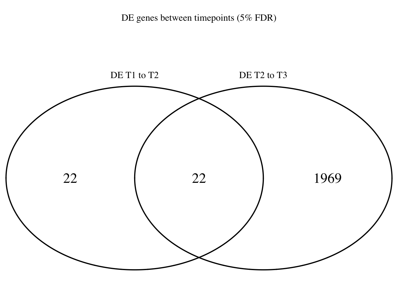

dev.off()

null device 
          1 

pdf(file = "~/Dropbox/Figures/DET1_T2_change_weight_FDR5.pdf")
  grid.draw(Four_comp)
dev.off()

null device 
          1 

Using DAVID

Step 1: Use awk command to go from annotation file to ENSG and gene name only

cat gencode.v22.annotation.gtf | awk ‘BEGIN{FS=“”}{split($9,a,“;”); if($3~“gene”) print a[1]“”a[3]“”$1“:”$4“-”$5“”$7}’ | sed ‘s/gene_id “//’ | sed ’s/gene_id”//’ | sed ‘s/gene_biotype “//’| sed ’s/gene_name”//’ | sed ’s/“//g’ > Homo_sapiens.GRCh38.v22_table.txt

Step 2: Get ENSEMBL Gene IDs for background

# Set FDR level

FDR_level <- 0.01

# Get gene names after filtering
genes=as.data.frame(rownames(counts_genes_in_cutoff))
colnames(genes) <- c("Gene_name")


# Gene to ID conversion document

gene_id <- read.table("../data/Homo_sapiens.GRCh38.v22_table.txt", stringsAsFactors = FALSE)
colnames(gene_id) <- c("ENSEMBL", "Gene_name")

# Eliminate the feature after the period (for DAVID)
check <- gsub("\\..*","",gene_id$ENSEMBL)

new_gene_id <- cbind(check, gene_id$Gene_name)
gene_id <- new_gene_id
colnames(gene_id) <- c("ENSEMBL", "Gene_name")

# Get gene names of the background
comb_background <- merge(genes, gene_id, by = c("Gene_name"))
summary(duplicated(comb_background$Gene_name))

   Mode   FALSE    TRUE 
logical   11616     387 

comb_background1 <- comb_background[!duplicated(comb_background$Gene_name),]

dim(comb_background1)

[1] 11616     2

#write.table(comb_background1$ENSEMBL, "../data/DAVID_background.txt", quote = F, row.names = F, col.names = F)

Step 3: Get ENSEMBL Gene IDs for T1 to T2 list

# Get gene names after filtering
genes=as.data.frame(rownames(Time1v2[which(Time1v2$adj.P.Val < FDR_level),]))

colnames(genes) <- c("Gene_name")

# Get gene names of the list
comb_list <- merge(genes, gene_id, by = c("Gene_name"))
summary(duplicated(comb_list$Gene_name))

   Mode 
logical 

comb_list <- comb_list[!duplicated(comb_list$Gene_name),]

dim(comb_list)

[1] 0 2

write.table(comb_list$ENSEMBL, "../data/DAVID_list_T1T2_weight.txt", quote = F, row.names = F, col.names = F)

# Kim et al used the top 100 genes

genes=as.data.frame(rownames(topTable(fit1, coef=1, adjust="BH", number=100, sort.by="T")))

colnames(genes) <- c("Gene_name")

# Get gene names of the list
comb_list <- merge(genes, gene_id, by = c("Gene_name"))
summary(duplicated(comb_list$Gene_name))

   Mode   FALSE 
logical     100 

comb_list <- comb_list[!duplicated(comb_list$Gene_name),]

dim(comb_list)

[1] 100   2

write.table(comb_list$ENSEMBL, "../data/DAVID_top100_list_T1T2_weight.txt", quote = F, row.names = F, col.names = F)

Step 4: Get ENSEMBL Gene IDs for T2 to T3 list

# Get gene names after filtering
genes=as.data.frame(rownames(Time2v3[which(Time2v3$adj.P.Val < FDR_level),]))

colnames(genes) <- c("Gene_name")

# Get gene names of the list
comb_list <- merge(genes, gene_id, by = c("Gene_name"))
summary(duplicated(comb_list$Gene_name))

   Mode   FALSE    TRUE 
logical     842       6 

comb_list <- comb_list[!duplicated(comb_list$Gene_name),]

dim(comb_list)

[1] 842   2

write.table(comb_list$ENSEMBL, "../data/DAVID_list_T2T3_weight.txt", quote = F, row.names = F, col.names = F)

# Kim et al used the top 100 genes

genes=as.data.frame(rownames(topTable(fit1, coef=2, adjust="BH", number=100, sort.by="T")))

colnames(genes) <- c("Gene_name")

# Get gene names of the list
comb_list <- merge(genes, gene_id, by = c("Gene_name"))
summary(duplicated(comb_list$Gene_name))

   Mode   FALSE    TRUE 
logical     100       1 

comb_list <- comb_list[!duplicated(comb_list$Gene_name),]

dim(comb_list)

[1] 100   2

write.table(comb_list$ENSEMBL, "../data/DAVID_top100_list_T2T3_weight.txt", quote = F, row.names = F, col.names = F)

Step 5: Upload or copy and paste the gene lists to DAVID at https://david.ncifcrf.gov/conversion.jsp. Note, larger gene lists are more likely to need to be copied and pasted in the “Upload” tab, rather than uploaded.

sessionInfo()

R version 3.4.3 (2017-11-30)
Platform: x86_64-apple-darwin15.6.0 (64-bit)
Running under: OS X El Capitan 10.11.6

Matrix products: default
BLAS: /Library/Frameworks/R.framework/Versions/3.4/Resources/lib/libRblas.0.dylib
LAPACK: /Library/Frameworks/R.framework/Versions/3.4/Resources/lib/libRlapack.dylib

locale:
[1] en_US.UTF-8/en_US.UTF-8/en_US.UTF-8/C/en_US.UTF-8/en_US.UTF-8

attached base packages:
[1] grid      stats     graphics  grDevices utils     datasets  methods  
[8] base     

other attached packages:
[1] cowplot_0.9.3       ggplot2_3.0.0       VennDiagram_1.6.20 
[4] futile.logger_1.4.3 edgeR_3.20.9        limma_3.34.9       

loaded via a namespace (and not attached):
 [1] Rcpp_0.12.18         bindr_0.1.1          compiler_3.4.3      
 [4] pillar_1.3.0         formatR_1.5          git2r_0.23.0        
 [7] plyr_1.8.4           workflowr_1.1.1      R.methodsS3_1.7.1   
[10] futile.options_1.0.1 R.utils_2.6.0        tools_3.4.3         
[13] digest_0.6.16        evaluate_0.11        tibble_1.4.2        
[16] gtable_0.2.0         lattice_0.20-35      pkgconfig_2.0.2     
[19] rlang_0.2.2          yaml_2.2.0           bindrcpp_0.2.2      
[22] withr_2.1.2          stringr_1.3.1        dplyr_0.7.6         
[25] knitr_1.20           tidyselect_0.2.4     locfit_1.5-9.1      
[28] rprojroot_1.3-2      glue_1.3.0           R6_2.2.2            
[31] rmarkdown_1.10       purrr_0.2.5          lambda.r_1.2.3      
[34] magrittr_1.5         whisker_0.3-2        backports_1.1.2     
[37] scales_1.0.0         htmltools_0.3.6      assertthat_0.2.0    
[40] colorspace_1.3-2     labeling_0.3         stringi_1.2.4       
[43] lazyeval_0.2.1       munsell_0.5.0        crayon_1.3.4        
[46] R.oo_1.22.0