<!DOCTYPE html> <html xmlns="http://www.w3.org/1999/xhtml"> <head> <meta charset="utf-8"> <meta http-equiv="Content-Type" content="text/html; charset=utf-8" /> <meta name="generator" content="pandoc" /> <meta name="author" content="Lei Sun" /> <meta name="date" content="2017-03-26" /> <title>Empirical Null with Gaussian Derivatives: Large Correlation</title> <script src="site_libs/jquery-1.11.3/jquery.min.js"></script> <meta name="viewport" content="width=device-width, initial-scale=1" /> <link href="site_libs/bootstrap-3.3.5/css/cosmo.min.css" rel="stylesheet" /> <script src="site_libs/bootstrap-3.3.5/js/bootstrap.min.js"></script> <script src="site_libs/bootstrap-3.3.5/shim/html5shiv.min.js"></script> <script src="site_libs/bootstrap-3.3.5/shim/respond.min.js"></script> <script src="site_libs/jqueryui-1.11.4/jquery-ui.min.js"></script> <link href="site_libs/tocify-1.9.1/jquery.tocify.css" rel="stylesheet" /> <script src="site_libs/tocify-1.9.1/jquery.tocify.js"></script> <script src="site_libs/navigation-1.1/tabsets.js"></script> <link href="site_libs/highlightjs-1.1/textmate.css" rel="stylesheet" /> <script src="site_libs/highlightjs-1.1/highlight.js"></script> <link href="site_libs/font-awesome-4.5.0/css/font-awesome.min.css" rel="stylesheet" /> <style type="text/css">code{white-space: pre;}</style> <style type="text/css"> pre:not([class]) { background-color: white; } </style> <script type="text/javascript"> if (window.hljs && document.readyState && document.readyState === "complete") { window.setTimeout(function() { hljs.initHighlighting(); }, 0); } </script> <style type="text/css"> h1 { font-size: 34px; } h1.title { font-size: 38px; } h2 { font-size: 30px; } h3 { font-size: 24px; } h4 { font-size: 18px; } h5 { font-size: 16px; } h6 { font-size: 12px; } .table th:not([align]) { text-align: left; } </style> </head> <body> <style type = "text/css"> .main-container { max-width: 940px; margin-left: auto; margin-right: auto; } code { color: inherit; background-color: rgba(0, 0, 0, 0.04); } img { max-width:100%; height: auto; } .tabbed-pane { padding-top: 12px; } button.code-folding-btn:focus { outline: none; } </style> <style type="text/css"> /* padding for bootstrap navbar */ body { padding-top: 51px; padding-bottom: 40px; } /* offset scroll position for anchor links (for fixed navbar) */ .section h1 { padding-top: 56px; margin-top: -56px; } .section h2 { padding-top: 56px; margin-top: -56px; } .section h3 { padding-top: 56px; margin-top: -56px; } .section h4 { padding-top: 56px; margin-top: -56px; } .section h5 { padding-top: 56px; margin-top: -56px; } .section h6 { padding-top: 56px; margin-top: -56px; } </style> <script> // manage active state of menu based on current page $(document).ready(function () { // active menu anchor href = window.location.pathname href = href.substr(href.lastIndexOf('/') + 1) if (href === "") href = "index.html"; var menuAnchor = $('a[href="' + href + '"]'); // mark it active menuAnchor.parent().addClass('active'); // if it's got a parent navbar menu mark it active as well menuAnchor.closest('li.dropdown').addClass('active'); }); </script> <div class="container-fluid main-container"> <!-- tabsets --> <script> $(document).ready(function () { window.buildTabsets("TOC"); }); </script> <!-- code folding --> <script> $(document).ready(function () { // move toc-ignore selectors from section div to header $('div.section.toc-ignore') .removeClass('toc-ignore') .children('h1,h2,h3,h4,h5').addClass('toc-ignore'); // establish options var options = { selectors: "h1,h2,h3", theme: "bootstrap3", context: '.toc-content', hashGenerator: function (text) { return text.replace(/[.\\/?&!#<>]/g, '').replace(/\s/g, '_').toLowerCase(); }, ignoreSelector: ".toc-ignore", scrollTo: 0 }; options.showAndHide = true; options.smoothScroll = true; // tocify var toc = $("#TOC").tocify(options).data("toc-tocify"); }); </script> <style type="text/css"> #TOC { margin: 25px 0px 20px 0px; } @media (max-width: 768px) { #TOC { position: relative; width: 100%; } } .toc-content { padding-left: 30px; padding-right: 40px; } div.main-container { max-width: 1200px; } div.tocify { width: 20%; max-width: 260px; max-height: 85%; } @media (min-width: 768px) and (max-width: 991px) { div.tocify { width: 25%; } } @media (max-width: 767px) { div.tocify { width: 100%; max-width: none; } } .tocify ul, .tocify li { line-height: 20px; } .tocify-subheader .tocify-item { font-size: 0.90em; padding-left: 25px; text-indent: 0; } .tocify .list-group-item { border-radius: 0px; } </style> <!-- setup 3col/9col grid for toc_float and main content --> <div class="row-fluid"> <div class="col-xs-12 col-sm-4 col-md-3"> <div id="TOC" class="tocify"> </div> </div> <div class="toc-content col-xs-12 col-sm-8 col-md-9"> <div class="navbar navbar-default navbar-fixed-top" role="navigation"> <div class="container"> <div class="navbar-header"> <button type="button" class="navbar-toggle collapsed" data-toggle="collapse" data-target="#navbar"> <span class="icon-bar"></span> <span class="icon-bar"></span> <span class="icon-bar"></span> </button> <a class="navbar-brand" href="index.html">truncash</a> </div> <div id="navbar" class="navbar-collapse collapse"> <ul class="nav navbar-nav"> <li> <a href="index.html">Home</a> </li> <li> <a href="about.html">About</a> </li> <li> <a href="license.html">License</a> </li> </ul> <ul class="nav navbar-nav navbar-right"> <li> <a href="https://github.com/LSun/truncash"> <span class="fa fa-github"></span> </a> </li> </ul> </div><!--/.nav-collapse --> </div><!--/.container --> </div><!--/.navbar --> <div class="fluid-row" id="header"> <h1 class="title toc-ignore">Empirical Null with Gaussian Derivatives: Large Correlation</h1> <h4 class="author"><em>Lei Sun</em></h4> <h4 class="date"><em>2017-03-26</em></h4> </div> <!-- The file analysis/chunks.R contains chunks that define default settings shared across the workflowr files. --> <!-- Update knitr chunk options --> <!-- Insert the date the file was last updated --> <!-- Insert the code version (Git commit SHA1) if Git repository exists and R package git2r is installed --> <!-- Add your analysis here --> <div id="can-k-be-too-small" class="section level2"> <h2>Can <span class="math inline">\(K\)</span> be too small?</h2> <p><a href="gaussian_derivatives.rmd">Another assumption</a> to make the problem tractable is that the pairwise correlation <span class="math inline">\(\rho_{ij}\)</span> is moderate enough so <span class="math inline">\(W_k\varphi^{(k)}\)</span> vanishes as the order <span class="math inline">\(k\)</span> increases. With this assumption we can stop at a sufficiently large <span class="math inline">\(K\)</span> without consideration higher order Gaussian derivatives. But what if <span class="math inline">\(\rho_{ij}\)</span> is large?</p> </div> <div id="extreme-case-rho_ij-equiv-1" class="section level2"> <h2>Extreme case: <span class="math inline">\(\rho_{ij} \equiv 1\)</span></h2> <p>When we have perfect correlation among all <span class="math inline">\(z\)</span> scores, the approximate limit observed density <span class="math inline">\(f_0(x)\to\delta_z(x) = \delta(x-z)\)</span>. That is, with probability one, we observe <span class="math inline">\(z_1 = \cdots = z_n = z\)</span>, as <span class="math inline">\(n\to\infty\)</span>, <span class="math inline">\(f_0(x)\)</span> goes to a Dirac delta function peak at the observed <span class="math inline">\(z\)</span>, and zero elsewhere. Now the question is, can this Dirac delta function be decomposed with the Gaussian <span class="math inline">\(\varphi\)</span> and its derivatives <span class="math inline">\(\varphi^{(k)}\)</span>, so that we still have</p> <p><span class="math display">\[ f_0(x) = \delta(x - z) = \varphi(x)\sum\limits_{k = 0}^\infty W_kh_k(x) \]</span> with appropriate <span class="math inline">\(W_k\)</span>’s?</p> <p>Using the orthogonality of Hermite functions, <a href="gaussian_derivatives.html#gaussian_derivatives_and_hermite_polynomials">we have</a></p> <p><span class="math display">\[ W_k = \frac{1}{k!}\int_{-\infty}^{\infty}h_k(x)f_0(x)dx = \frac{1}{k!}\int_{-\infty}^{\infty}h_k(x)\delta(x-z)dx = \frac{1}{k!}h_k(z) \]</span> Now the decomposition <span class="math inline">\(\varphi(x)\sum\limits_{k = 0}^\infty W_kh_k(x)\)</span> becomes</p> <p><span class="math display">\[ \varphi(x)\sum\limits_{k = 0}^\infty \frac{1}{k!}h_k(z)h_k(x) \]</span> It turns out this equation is connected to <a href="https://en.wikipedia.org/wiki/Mehler_kernel">Mehler’s formula</a> which can be <a href="https://en.wikipedia.org/wiki/Hermite_polynomials#Completeness_relation">shown</a> to give the identity</p> <p><span class="math display">\[ \sum\limits_{k = 0}^\infty \psi_k(x)\psi_k(z) = \delta(x - z) \]</span> where <span class="math inline">\(\psi_k\)</span>’s are the <a href="https://en.wikipedia.org/wiki/Hermite_polynomials#Hermite_functions">Hermite functions</a> defined as</p> <p><span class="math display">\[ \begin{array}{rrcl} & \psi_k(x) &=& (k!)^{-1/2}(\sqrt{\pi})^{-1/2}e^{-x^2/2}h_k(\sqrt{2}x)\\ \Rightarrow & h_k(x) &=& (k!)^{1/2}(\sqrt{\pi})^{1/2}e^{x^2/4}\psi_k\left(\frac x{\sqrt{2}}\right)\\ \Rightarrow & \varphi(x)\sum\limits_{k = 0}^\infty \frac{1}{k!}h_k(z)h_k(x) & =& \frac1{\sqrt{2}}e^{-\frac{x^2}4+\frac{z^2}4}\sum\limits_{k = 0}^\infty \psi_k\left(\frac x{\sqrt{2}}\right)\psi_k\left(\frac z{\sqrt{2}}\right)\\ & &=& \frac1{\sqrt{2}}e^{-\frac{x^2}4+\frac{z^2}4} \delta\left(\frac{x - z}{\sqrt{2}}\right) \end{array} \]</span> Note that the Dirac delta function has a property that <span class="math inline">\(\delta(\alpha x) = \delta(x) / |\alpha| \Rightarrow \frac1{\sqrt{2}}\delta\left(\frac{x - z}{\sqrt{2}}\right) = \delta(x - z)\)</span>. Therefore,</p> <p><span class="math display">\[ \varphi(x)\sum\limits_{k = 0}^\infty \frac{1}{k!}h_k(z)h_k(x) = \delta(x-z)\exp\left(-\frac{x^2}4+\frac{z^2}4\right) \]</span> Note that <span class="math inline">\(\exp\left(-\frac{x^2}4+\frac{z^2}4\right)\)</span> is bounded for any <span class="math inline">\(z\in\mathbb{R}\)</span>, so <span class="math inline">\(\delta(x-z)\exp\left(-\frac{x^2}4+\frac{z^2}4\right)\)</span> vanishes to <span class="math inline">\(0\)</span> for any <span class="math inline">\(x\neq z\)</span>, and</p> <p><span class="math display">\[ \int_{-\infty}^\infty \delta(x-z)\exp\left(-\frac{x^2}4+\frac{z^2}4\right)dx = \exp\left(-\frac{z^2}4+\frac{z^2}4\right) = 1 \]</span> Hence, in essence, <span class="math inline">\(\delta(x-z)\exp\left(-\frac{x^2}4+\frac{z^2}4\right) = \delta(x-z)\)</span>. Therefore we have <span class="math display">\[ f_0(x) = \varphi(x)\sum\limits_{k = 0}^\infty W_kh_k(x) = \varphi(x)\sum\limits_{k = 0}^\infty \frac{1}{k!}h_k(z)h_k(x) =\delta(x -z) \]</span> when <span class="math display">\[ W_k = \frac{1}{k!}h_k(z) \]</span> Thus we show that the Dirac delta function can be decomposed by Gaussian density and its derivatives.</p> <div id="visualization-with-finite-k" class="section level3"> <h3>Visualization with finite <span class="math inline">\(K\)</span></h3> <p>With Gaussian and its infinite orders of derivatives, we can compose a Dirac delta function at any position, yet what happens if we stop at a finite <span class="math inline">\(K\)</span>? Let <span class="math inline">\(f_0^K\)</span> be the approximation of <span class="math inline">\(f_0 = \delta_z\)</span> with first <span class="math inline">\(K\)</span> Gaussian derivatives. That is,</p> <p><span class="math display">
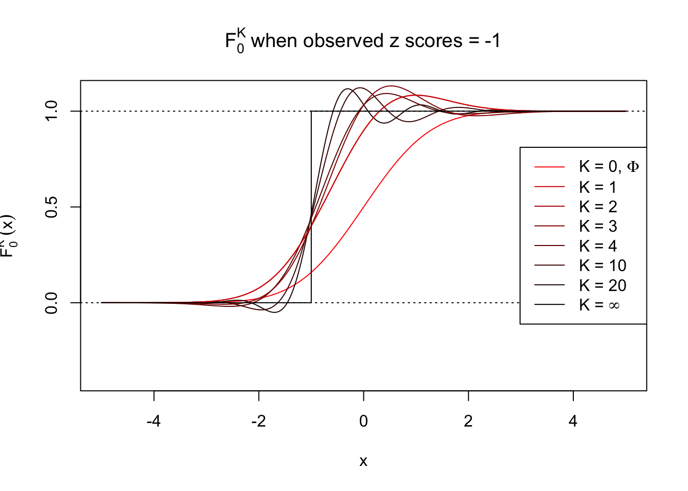
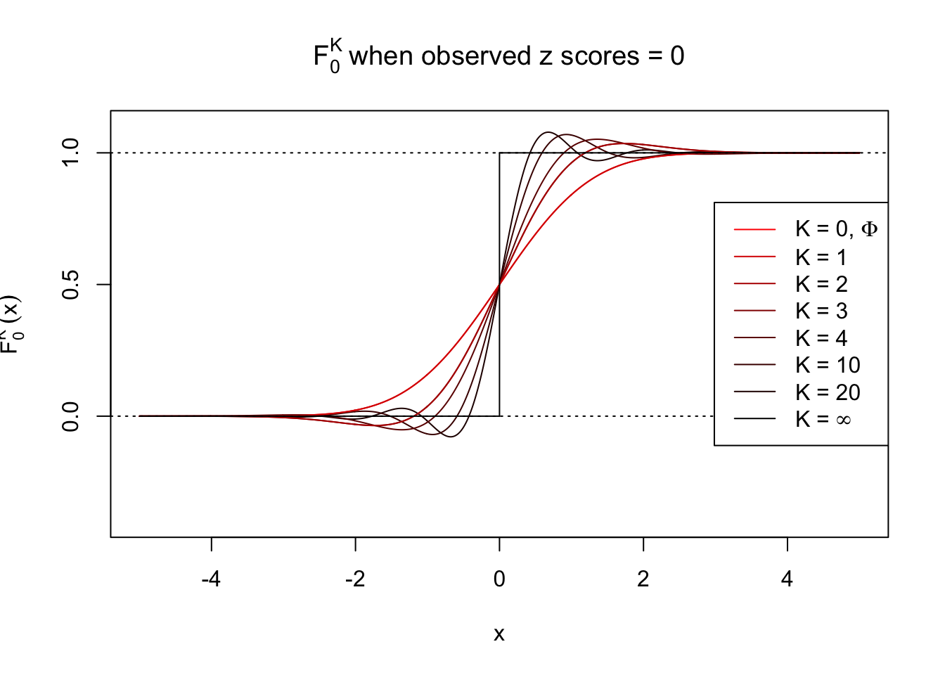
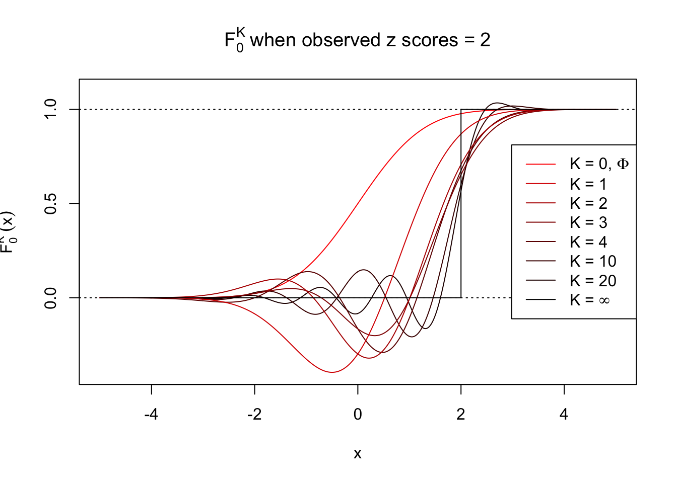
\[ f_0^K(x) = \varphi(x)\sum\limits_{k = 0}^K \frac{1}{k!}h_k(z)h_k(x) \ . \]</span> Meanwhile, let <span class="math inline">\(F_0^K(x) = \int_{-\infty}^x f_0^K(u)du\)</span>. It’s easy to shown that</p> <p><span class="math display">\[ F_0^K(x) = \Phi(x) - \varphi(x)\sum\limits_{k = 1}^K W_k h_{k - 1}(x) = \Phi(x) - \varphi(x) \sum\limits_{k = 1}^K \frac{1}{k!}h_k(z) h_{k - 1}(x) \ . \]</span></p> <p>Theoretically, <span class="math inline">\(f_0^K\)</span> is an approximation to empirical density of perfectly correlated <span class="math inline">\(z\)</span> scores; hence, as <span class="math inline">\(K\to\infty\)</span>, <span class="math inline">\(f_0^K\to\delta_z\)</span>. Similarly, <span class="math inline">\(F_0^K\)</span> is an approximation to empirical cdf of perfectly correlated <span class="math inline">\(z\)</span> scores; hence, as <span class="math inline">\(K\to\infty\)</span>, <span class="math inline">\(f_0^K\)</span> should converge to the <span class="math inline">\(0\)</span>-<span class="math inline">\(1\)</span> step function, and the location of the step is the observed <span class="math inline">\(z\)</span>.</p> <p>In practice, the convergence is not fast. As we can see from the following visualization, the difference between <span class="math inline">\(f_0^K\)</span> and <span class="math inline">\(\delta_z\)</span>, as well as that between <span class="math inline">\(F_0^K\)</span> and the step function, is still conspicuous even if <span class="math inline">\(K = 20\)</span>, which is about the highest order <code>R</code> can reasonbly handle in the current implementation. Therefore, at least in theory it’s possible that <span class="math inline">\(K\)</span> can be too small.</p> <p><strong>Note that the oscillation near the presumptive step may be connected with <a href="https://en.wikipedia.org/wiki/Gibbs_phenomenon">Gibbs phenomenon</a>.</strong></p> <pre><code>Under perfect correlation, observed z scores = -1 </code></pre> <p><img src="figure/gaussian_derivatives_4.rmd/unnamed-chunk-2-1.png" width="672" style="display: block; margin: auto;" /><img src="figure/gaussian_derivatives_4.rmd/unnamed-chunk-2-2.png" width="672" style="display: block; margin: auto;" /></p> <pre><code>
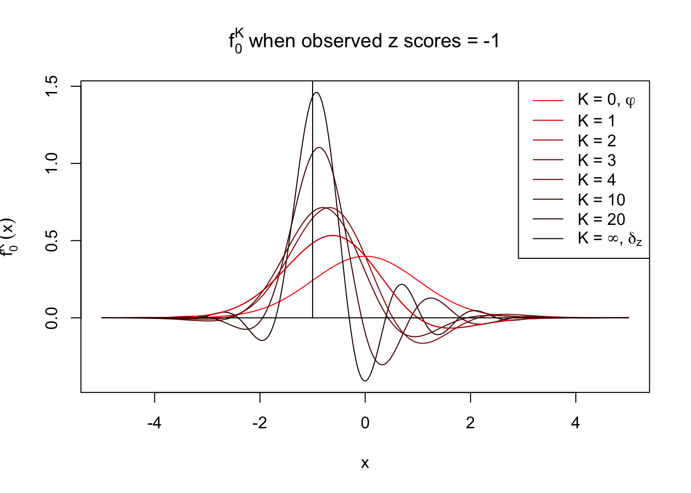
Under perfect correlation, observed z scores = 0 </code></pre> <p><img src="figure/gaussian_derivatives_4.rmd/unnamed-chunk-2-3.png" width="672" style="display: block; margin: auto;" /><img src="figure/gaussian_derivatives_4.rmd/unnamed-chunk-2-4.png" width="672" style="display: block; margin: auto;" /></p> <pre><code>
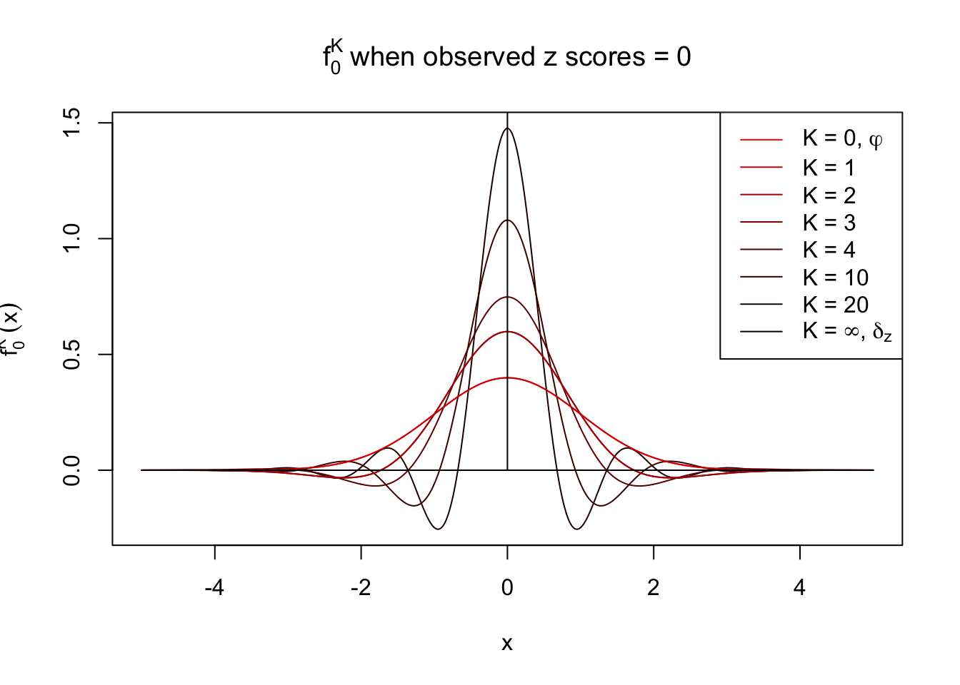
Under perfect correlation, observed z scores = 2
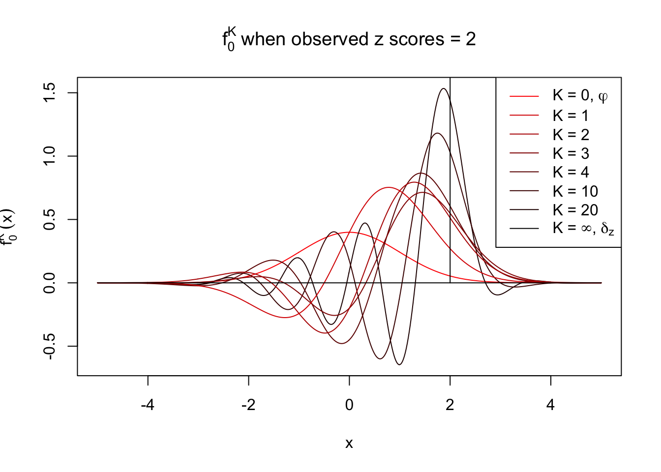
 </code></pre> <p><img src="figure/gaussian_derivatives_4.rmd/unnamed-chunk-2-5.png" width="672" style="display: block; margin: auto;" /><img src="figure/gaussian_derivatives_4.rmd/unnamed-chunk-2-6.png" width="672" style="display: block; margin: auto;" /></p> </div> </div> <div id="fitting-experiments-when-rho_ij-is-large" class="section level2"> <h2>Fitting experiments when <span class="math inline">\(\rho_{ij}\)</span> is large</h2> <p>As previous theoretical result indicates, when <span class="math inline">\(\rho\)</span> is large, a large <span class="math inline">\(K\)</span> is probably needed. However, on the other hand, when <span class="math inline">\(\rho\)</span> is large, the effective sample size is small. Indeed when <span class="math inline">\(\rho\equiv1\)</span>, the sample size is essentially <span class="math inline">\(1\)</span>.</p> <p>Let’s take a look at some examples with pairwise correlations of <span class="math inline">\(z\)</span> scores <span class="math inline">\(\rho_{ij}\equiv\rho\)</span>, <span class="math inline">\(\rho\)</span> moderate to high. Such <span class="math inline">\(z\)</span> scores can be simulated as <span class="math inline">\(z_i = \epsilon\sqrt{\rho} + e_i\sqrt{1-\rho}\)</span>, where <span class="math inline">\(\epsilon, e_i\)</span> are iid <span class="math inline">\(N(0, 1)\)</span>.</p> <pre class="r"><code>n = 1e4 rho = 0.5 set.seed(777) z = rnorm(1) * sqrt(rho) + rnorm(n) * sqrt(1 - rho)</code></pre> <pre class="r"><code>source("../code/ecdfz.R") fit.ecdfz = ecdfz.optimal(z)</code></pre> <p>When <span class="math inline">\(\rho = 0.5\)</span>, current implementation with <span class="math inline">\(K = 5\)</span> fits positively correlationed z scores reasonably well.</p> <pre><code>10000 z scores with pairwise correlation = 0.5
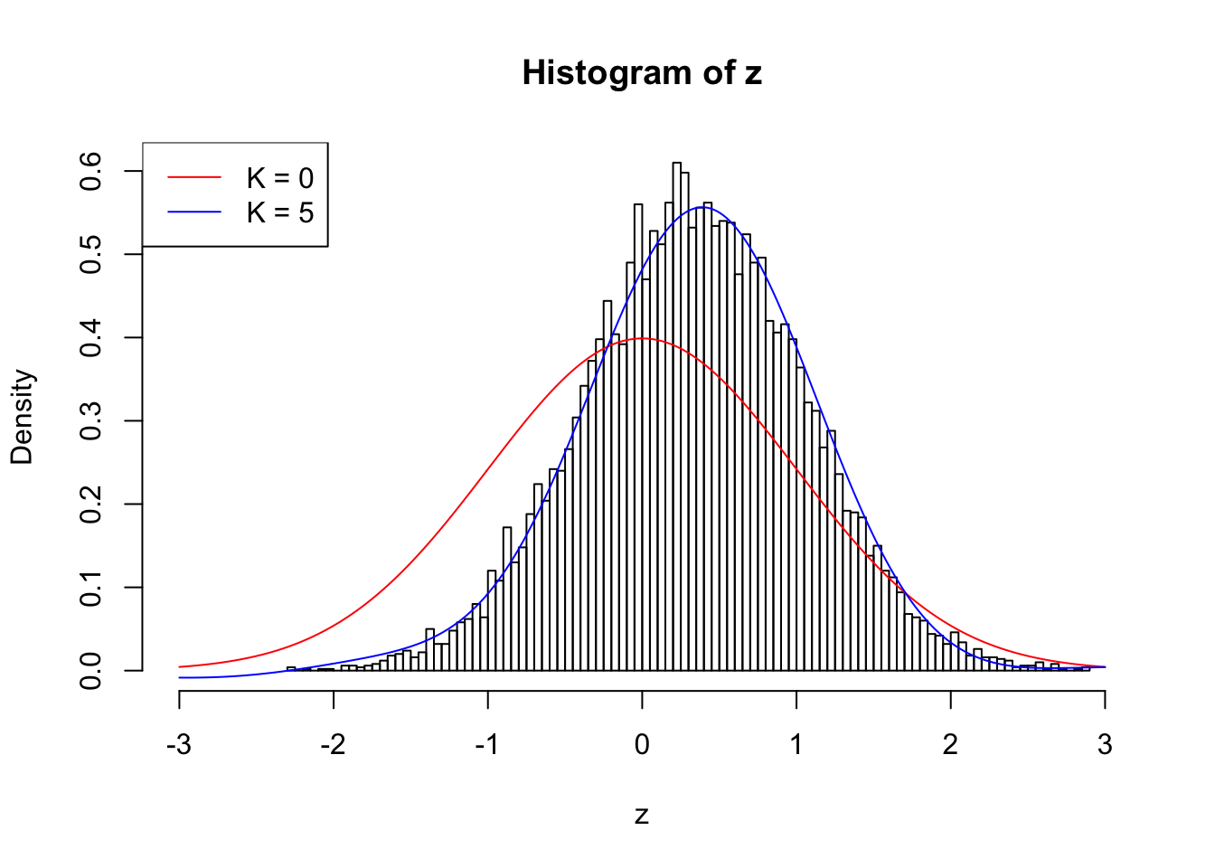
</code></pre> <p><img src="figure/gaussian_derivatives_4.rmd/unnamed-chunk-6-1.png" width="672" style="display: block; margin: auto;" /></p> <p>However, as <span class="math inline">\(\rho\)</span> gets larger, current implementation usually fails to find a good <span class="math inline">\(K\)</span> before the algorithm goes unstable, as illustrated in the following <span class="math inline">\(\rho = 0.7\)</span> plot. <span class="math inline">\(K = 3\)</span> is obviously not enough, yet <span class="math inline">\(K = 4\)</span> has already gone wildly unstable.</p> <pre class="r"><code>n = 1e4 rho = 0.7 set.seed(777) z = rnorm(1) * sqrt(rho) + rnorm(n) * sqrt(1 - rho)</code></pre> <pre class="r"><code>source("../code/ecdfz.R") fit.ecdfz = ecdfz.optimal(z)</code></pre> <pre><code>10000 z scores with pairwise correlation = 0.7
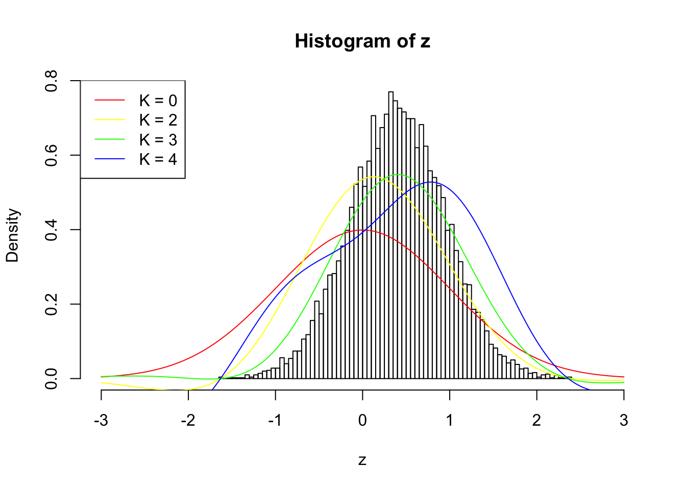
</code></pre> <p><img src="figure/gaussian_derivatives_4.rmd/unnamed-chunk-9-1.png" width="672" style="display: block; margin: auto;" /></p> <p>When <span class="math inline">\(\rho = 0.9\)</span>, the observed <span class="math inline">\(z\)</span> scores are so concentrated in a small range, even if we have <span class="math inline">\(10,000\)</span> of them, making the effective sample size hopelessly small. Current implementation can’t even handle this data set; it goes crazy when <span class="math inline">\(K = 2\)</span>.</p> <pre class="r"><code>n = 1e4 rho = 0.9 set.seed(777) z = rnorm(1) * sqrt(rho) + rnorm(n) * sqrt(1 - rho)</code></pre> <pre class="r"><code>source("../code/ecdfz.R") fit.ecdfz = ecdfz(z, 2)</code></pre> <pre><code>10000 z scores with pairwise correlation = 0.9
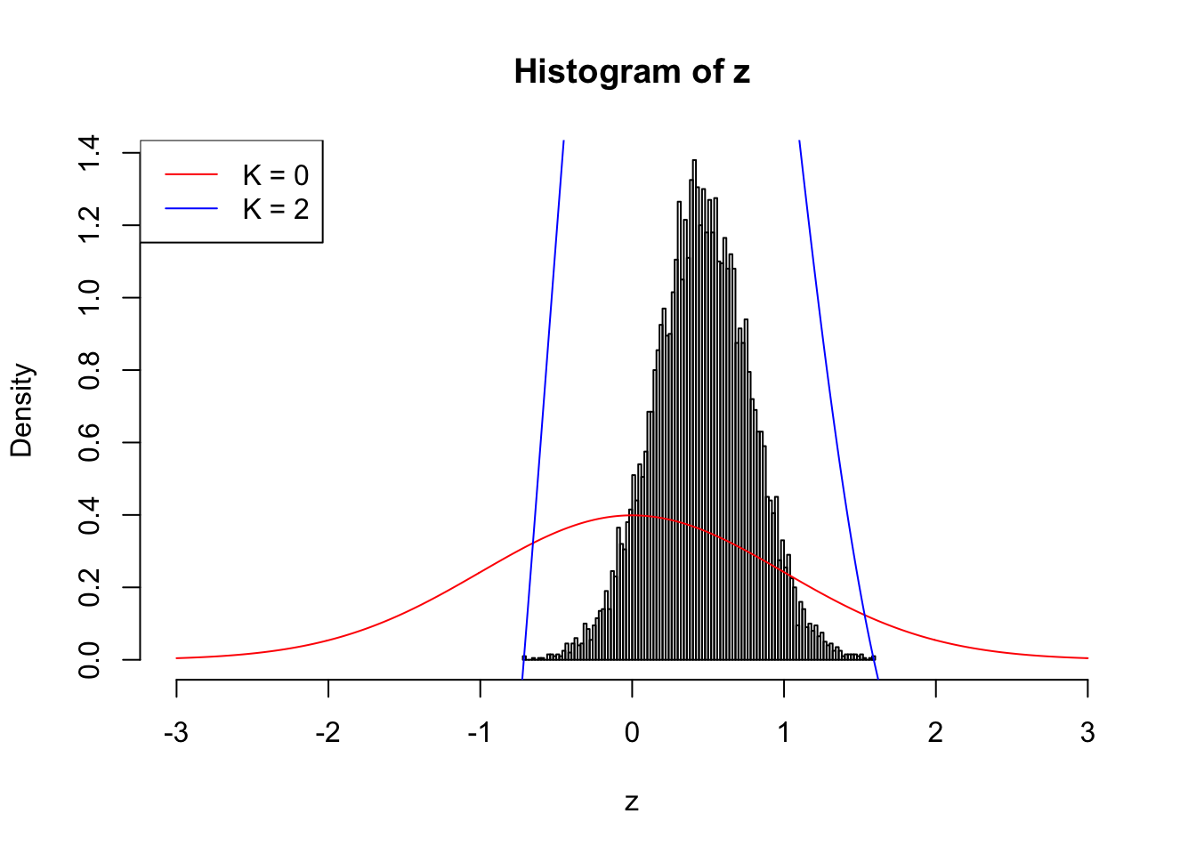
</code></pre> <p><img src="figure/gaussian_derivatives_4.rmd/unnamed-chunk-12-1.png" width="672" style="display: block; margin: auto;" /></p> </div> <div id="session-information" class="section level2"> <h2>Session information</h2> <!-- Insert the session information into the document --> <pre class="r"><code>sessionInfo()</code></pre> <pre><code>R version 3.3.2 (2016-10-31) Platform: x86_64-apple-darwin13.4.0 (64-bit) Running under: macOS Sierra 10.12.3 locale: [1] en_US.UTF-8/en_US.UTF-8/en_US.UTF-8/C/en_US.UTF-8/en_US.UTF-8 attached base packages: [1] stats graphics grDevices utils datasets methods base loaded via a namespace (and not attached): [1] backports_1.0.5 magrittr_1.5 rprojroot_1.2 tools_3.3.2 [5] htmltools_0.3.5 yaml_2.1.14 Rcpp_0.12.10 stringi_1.1.2 [9] rmarkdown_1.3 knitr_1.15.1 stringr_1.1.0 digest_0.6.9 [13] evaluate_0.10 </code></pre> </div> <hr> <p> This <a href="http://rmarkdown.rstudio.com">R Markdown</a> site was created with <a href="https://github.com/jdblischak/workflowr">workflowr</a> </p> <hr> <!-- To enable disqus, uncomment the section below and provide your disqus_shortname --> <!-- disqus <div id="disqus_thread"></div> <script type="text/javascript"> /* * * CONFIGURATION VARIABLES: EDIT BEFORE PASTING INTO YOUR WEBPAGE * * */ var disqus_shortname = 'rmarkdown'; // required: replace example with your forum shortname /* * * DON'T EDIT BELOW THIS LINE * * */ (function() { var dsq = document.createElement('script'); dsq.type = 'text/javascript'; dsq.async = true; dsq.src = '//' + disqus_shortname + '.disqus.com/embed.js'; (document.getElementsByTagName('head')[0] || document.getElementsByTagName('body')[0]).appendChild(dsq); })(); </script> <noscript>Please enable JavaScript to view the <a href="http://disqus.com/?ref_noscript">comments powered by Disqus.</a></noscript> <a href="http://disqus.com" class="dsq-brlink">comments powered by <span class="logo-disqus">Disqus</span></a> --> </div> </div> </div> <script> // add bootstrap table styles to pandoc tables function bootstrapStylePandocTables() { $('tr.header').parent('thead').parent('table').addClass('table table-condensed'); } $(document).ready(function () { bootstrapStylePandocTables(); }); </script> <!-- dynamically load mathjax for compatibility with self-contained --> <script> (function () { var script = document.createElement("script"); script.type = "text/javascript"; script.src = "https://cdn.mathjax.org/mathjax/latest/MathJax.js?config=TeX-AMS-MML_HTMLorMML"; document.getElementsByTagName("head")[0].appendChild(script); })(); </script> </body> </html>