The Distribution of \(W_j\)
Lei Sun
2018-04-13
Last updated: 2018-06-10
workflowr checks: (Click a bullet for more information)-
✔ R Markdown file: up-to-date
Great! Since the R Markdown file has been committed to the Git repository, you know the exact version of the code that produced these results.
-
✔ Environment: empty
Great job! The global environment was empty. Objects defined in the global environment can affect the analysis in your R Markdown file in unknown ways. For reproduciblity it’s best to always run the code in an empty environment.
-
✔ Seed:
set.seed(12345)The command
set.seed(12345)was run prior to running the code in the R Markdown file. Setting a seed ensures that any results that rely on randomness, e.g. subsampling or permutations, are reproducible. -
✔ Session information: recorded
Great job! Recording the operating system, R version, and package versions is critical for reproducibility.
-
Great! You are using Git for version control. Tracking code development and connecting the code version to the results is critical for reproducibility. The version displayed above was the version of the Git repository at the time these results were generated.✔ Repository version: 386b1fd
Note that you need to be careful to ensure that all relevant files for the analysis have been committed to Git prior to generating the results (you can usewflow_publishorwflow_git_commit). workflowr only checks the R Markdown file, but you know if there are other scripts or data files that it depends on. Below is the status of the Git repository when the results were generated:
Note that any generated files, e.g. HTML, png, CSS, etc., are not included in this status report because it is ok for generated content to have uncommitted changes.Ignored files: Ignored: .DS_Store Ignored: .Rhistory Ignored: .Rproj.user/ Ignored: analysis/.DS_Store Ignored: analysis/BH_robustness_cache/ Ignored: analysis/FDR_Null_cache/ Ignored: analysis/FDR_null_betahat_cache/ Ignored: analysis/Rmosek_cache/ Ignored: analysis/StepDown_cache/ Ignored: analysis/alternative2_cache/ Ignored: analysis/alternative_cache/ Ignored: analysis/ash_gd_cache/ Ignored: analysis/average_cor_gtex_2_cache/ Ignored: analysis/average_cor_gtex_cache/ Ignored: analysis/brca_cache/ Ignored: analysis/cash_deconv_cache/ Ignored: analysis/cash_fdr_1_cache/ Ignored: analysis/cash_fdr_2_cache/ Ignored: analysis/cash_fdr_3_cache/ Ignored: analysis/cash_fdr_4_cache/ Ignored: analysis/cash_fdr_5_cache/ Ignored: analysis/cash_fdr_6_cache/ Ignored: analysis/cash_plots_2_cache/ Ignored: analysis/cash_plots_cache/ Ignored: analysis/cash_sim_1_cache/ Ignored: analysis/cash_sim_2_cache/ Ignored: analysis/cash_sim_3_cache/ Ignored: analysis/cash_sim_4_cache/ Ignored: analysis/cash_sim_5_cache/ Ignored: analysis/cash_sim_6_cache/ Ignored: analysis/cash_sim_7_cache/ Ignored: analysis/correlated_z_2_cache/ Ignored: analysis/correlated_z_3_cache/ Ignored: analysis/correlated_z_cache/ Ignored: analysis/create_null_cache/ Ignored: analysis/cutoff_null_cache/ Ignored: analysis/design_matrix_2_cache/ Ignored: analysis/design_matrix_cache/ Ignored: analysis/diagnostic_ash_cache/ Ignored: analysis/diagnostic_correlated_z_2_cache/ Ignored: analysis/diagnostic_correlated_z_3_cache/ Ignored: analysis/diagnostic_correlated_z_cache/ Ignored: analysis/diagnostic_plot_2_cache/ Ignored: analysis/diagnostic_plot_cache/ Ignored: analysis/efron_leukemia_cache/ Ignored: analysis/figure/ Ignored: analysis/fitting_normal_cache/ Ignored: analysis/gaussian_derivatives_2_cache/ Ignored: analysis/gaussian_derivatives_3_cache/ Ignored: analysis/gaussian_derivatives_4_cache/ Ignored: analysis/gaussian_derivatives_5_cache/ Ignored: analysis/gaussian_derivatives_cache/ Ignored: analysis/gd-ash_cache/ Ignored: analysis/gd_delta_cache/ Ignored: analysis/gd_lik_2_cache/ Ignored: analysis/gd_lik_cache/ Ignored: analysis/gd_w_cache/ Ignored: analysis/knockoff_10_cache/ Ignored: analysis/knockoff_2_cache/ Ignored: analysis/knockoff_3_cache/ Ignored: analysis/knockoff_4_cache/ Ignored: analysis/knockoff_5_cache/ Ignored: analysis/knockoff_6_cache/ Ignored: analysis/knockoff_7_cache/ Ignored: analysis/knockoff_8_cache/ Ignored: analysis/knockoff_9_cache/ Ignored: analysis/knockoff_cache/ Ignored: analysis/knockoff_var_cache/ Ignored: analysis/marginal_z_alternative_cache/ Ignored: analysis/marginal_z_cache/ Ignored: analysis/mosek_reg_2_cache/ Ignored: analysis/mosek_reg_4_cache/ Ignored: analysis/mosek_reg_5_cache/ Ignored: analysis/mosek_reg_6_cache/ Ignored: analysis/mosek_reg_cache/ Ignored: analysis/pihat0_null_cache/ Ignored: analysis/plot_diagnostic_cache/ Ignored: analysis/poster_obayes17_cache/ Ignored: analysis/real_data_simulation_2_cache/ Ignored: analysis/real_data_simulation_3_cache/ Ignored: analysis/real_data_simulation_4_cache/ Ignored: analysis/real_data_simulation_5_cache/ Ignored: analysis/real_data_simulation_cache/ Ignored: analysis/rmosek_primal_dual_2_cache/ Ignored: analysis/rmosek_primal_dual_cache/ Ignored: analysis/seqgendiff_cache/ Ignored: analysis/simulated_correlated_null_2_cache/ Ignored: analysis/simulated_correlated_null_3_cache/ Ignored: analysis/simulated_correlated_null_cache/ Ignored: analysis/simulation_real_se_2_cache/ Ignored: analysis/simulation_real_se_cache/ Ignored: analysis/smemo_2_cache/ Ignored: data/LSI/ Ignored: docs/.DS_Store Ignored: docs/figure/.DS_Store Ignored: output/fig/
Expand here to see past versions:
| File | Version | Author | Date | Message |
|---|---|---|---|---|
| rmd | 386b1fd | LSun | 2018-06-10 | wflow_publish(“analysis/gd_w.rmd”) |
| rmd | d8add67 | Lei Sun | 2018-06-10 | selected examples |
| html | ff560a1 | LSun | 2018-06-10 | Build site. |
| rmd | dc80048 | Lei Sun | 2018-06-09 | gene random |
| rmd | ee5f1d8 | LSun | 2018-06-09 | GD |
| html | b0f5a28 | LSun | 2018-06-03 | Build site. |
| rmd | 7f9e4ff | LSun | 2018-06-03 | wflow_publish(“analysis/gd_w.rmd”) |
| html | 792751b | LSun | 2018-06-02 | Build site. |
| rmd | b7bf225 | Lei Sun | 2018-06-02 | ecdf.avg |
| html | cf1e8e9 | LSun | 2018-06-01 | Build site. |
| rmd | 08b81b6 | LSun | 2018-06-01 | wflow_publish(“analysis/gd_w.rmd”) |
| html | b4bd5d8 | LSun | 2018-05-30 | Build site. |
| rmd | edfa8ce | Lei Sun | 2018-05-30 | new KM |
| html | 086abd6 | LSun | 2018-05-30 | Build site. |
| rmd | e9c3b2d | LSun | 2018-05-30 | wflow_publish(“analysis/gd_w.rmd”) |
| html | 99004e9 | LSun | 2018-05-30 | Build site. |
| rmd | d54a155 | Lei Sun | 2018-05-30 | eps |
| html | 2acb1ab | LSun | 2018-05-29 | Build site. |
| rmd | fc26405 | Lei Sun | 2018-05-29 | revision |
| html | b42a125 | LSun | 2018-05-29 | Build site. |
| rmd | c1f43e0 | LSun | 2018-05-29 | wflow_publish(“analysis/gd_w.rmd”) |
| rmd | 1ca47ca | Lei Sun | 2018-05-29 | revise |
| rmd | 119caf9 | LSun | 2018-05-29 | deconv |
| rmd | 2716923 | Lei Sun | 2018-05-29 | deconv |
| html | 9914885 | LSun | 2018-05-27 | Build site. |
| rmd | e68958a | Lei Sun | 2018-05-27 | fit |
| html | fd44b58 | LSun | 2018-05-26 | Build site. |
| rmd | 572e589 | Lei Sun | 2018-05-26 | plots |
| rmd | bb57226 | Lei Sun | 2018-05-26 | plots |
| rmd | 854ec31 | Lei Sun | 2018-05-26 | plots |
| rmd | 9b26932 | Lei Sun | 2018-05-26 | plots |
| rmd | 086a2bf | Lei Sun | 2018-05-26 | output |
| rmd | 14d847a | Lei Sun | 2018-05-26 | histograms of z |
| html | 7b21d1f | LSun | 2018-05-25 | Build site. |
| rmd | 535ecdd | LSun | 2018-05-25 | wflow_publish(“analysis/gd_w.rmd”) |
| html | 4d653b1 | LSun | 2018-05-15 | Build site. |
| html | e05bc83 | LSun | 2018-05-12 | Update to 1.0 |
| rmd | cc0ab83 | Lei Sun | 2018-05-11 | update |
| html | 807f924 | LSun | 2018-05-11 | Build site. |
| rmd | 548070e | LSun | 2018-05-11 | wflow_publish(“analysis/gd_w.rmd”) |
| html | 84c7d5b | LSun | 2018-05-11 | Build site. |
| rmd | 5c9aeac | LSun | 2018-05-11 | wflow_publish(“analysis/gd_w.rmd”) |
| html | ed9c0d9 | LSun | 2018-05-11 | Build site. |
| rmd | 0ea9f77 | Lei Sun | 2018-05-10 | W |
| html | adeab80 | LSun | 2018-05-06 | Build site. |
| rmd | 0b0a394 | LSun | 2018-05-06 | wflow_publish(c(“analysis/BH_robustness.rmd”, “analysis/gd_w.rmd”)) |
| html | 720d179 | LSun | 2018-04-18 | Build site. |
| rmd | b82e2bc | LSun | 2018-04-18 | wflow_publish(c(“analysis/gd_w.rmd”, “analysis/index.Rmd”)) |
| rmd | c7c5984 | Lei Sun | 2018-04-15 | ecdfz |
| html | 1c2f32e | LSun | 2018-04-15 | Build site. |
| rmd | 3b5dcc4 | LSun | 2018-04-15 | wflow_publish(“analysis/gd_w.rmd”) |
| rmd | 1b5d40f | Lei Sun | 2018-04-13 | gd w |
| rmd | c766b80 | LSun | 2018-04-13 | add lfsr |
source("../code/gdash_lik.R")Warning: package 'Matrix' was built under R version 3.4.4source("../code/gdfit.R")
source("../code/count_to_summary.R")
library(limma)
library(edgeR)
library(ashr)
library(plyr)
library(ggplot2)
library(reshape2)
library(decon)
library(deconvolveR)Introduction
Simulated Data
set.seed(777)
d <- 10
n <- 1e4
B <- matrix(rnorm(n * d), n, d)
Sigma <- B %*% t(B) + diag(n)
sigma <- diag(Sigma)
Rho <- cov2cor(Sigma)
rhobar <- c()
for (l in 1 : 10) {
  rhobar[l] <- (sum(Rho^l) - n) / (n * (n - 1))
}
par(mar = c(5.1, 4.1, 1, 2.1))
hist(Rho[lower.tri(Rho)], xlab = expression(rho[ij]), main = "")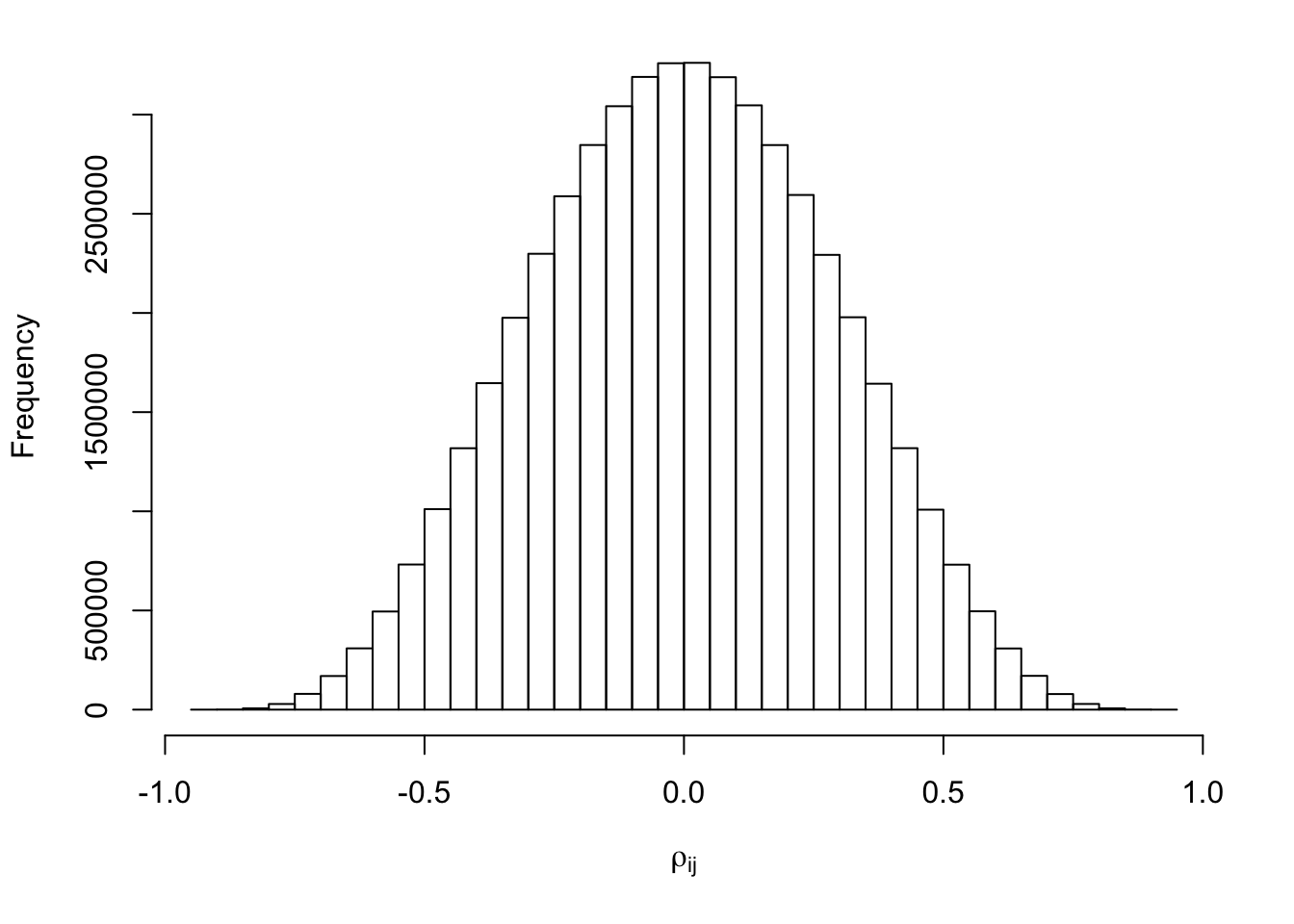
Expand here to see past versions of unnamed-chunk-3-1.png:
| Version | Author | Date |
|---|---|---|
| 720d179 | LSun | 2018-04-18 |
set.seed(20)
z <- rnorm(d)
Z <- B %*% z + rnorm(n)
Z <- Z / sqrt(sigma)
cat("sd(Z) =", sd(Z))
sd(Z) = 1.262205hist(Z, breaks = 20, prob = TRUE, ylim = c(0, dnorm(0)))
lines(seq(-5, 5, by = 0.1), dnorm(seq(-5, 5, by = 0.1)), col = "blue")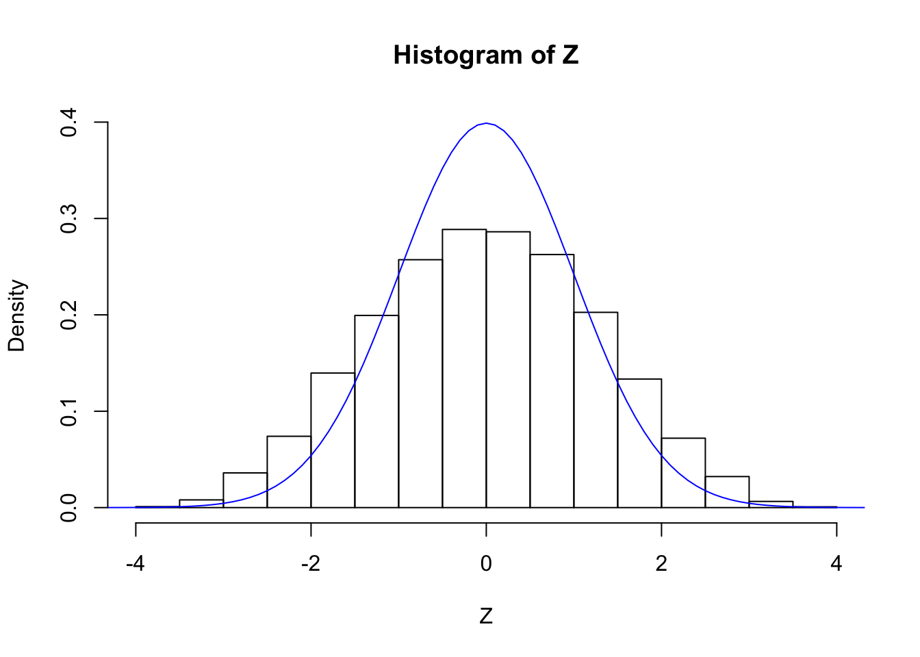
Expand here to see past versions of unnamed-chunk-4-1.png:
| Version | Author | Date |
|---|---|---|
| 720d179 | LSun | 2018-04-18 |
p <- pnorm(-abs(Z)) * 2

par(mfcol = c(2, 2))
par(mar = c(5.1, 4.1, 3, 2.1))
hist(p, breaks = 100, main = "Correlated", xlab = "p-value")

par(mar = c(5.1, 4.1, 1, 2.1))
plot(-log(p), ylim = range(-log(p), -log(pnorm(-sqrt(2 * log(n))) * 2), -log(0.05 / n)))
abline(h = -log(pnorm(-sqrt(2 * log(n))) * 2), col = "maroon")
abline(h = -log(0.05 / n), col = "red")
abline(h = -log(0.001), col = "green")
abline(h = -log(0.05), col = "blue")

Z <- rnorm(n)
p <- pnorm(-abs(Z)) * 2
par(mar = c(5.1, 4.1, 3, 2.1))
hist(p, breaks = 100, main = "Independent", xlab = "p-value")

par(mar = c(5.1, 4.1, 1, 2.1))
plot(-log(p), ylim = range(-log(p), -log(pnorm(-sqrt(2 * log(n))) * 2), -log(0.05 / n)))
abline(h = -log(pnorm(-sqrt(2 * log(n))) * 2), col = "maroon")
abline(h = -log(0.05 / n), col = "red")
abline(h = -log(0.001), col = "green")
abline(h = -log(0.05), col = "blue")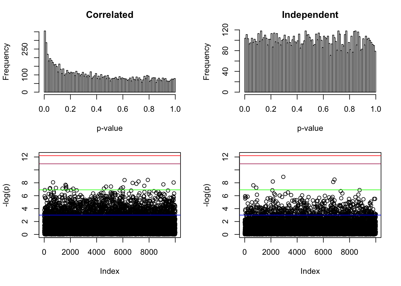
Expand here to see past versions of unnamed-chunk-4-2.png:
| Version | Author | Date |
|---|---|---|
| 720d179 | LSun | 2018-04-18 |
set.seed(777)
nsim <- 1e4
Z.list <- W <- list()
for (i in 1 : nsim) {
z <- rnorm(d)
Z <- B %*% z + rnorm(n)
Z <- Z / sqrt(sigma)
Z.list[[i]] <- Z
Z.GD <- gdfit.mom(Z, 100)
W[[i]] <- Z.GD$w
}
Z.sim <- Z.list
W.sim <- W
Real Data from GTEx
r <- readRDS("../data/liver.rds")top_genes_index = function (g, X) {
return(order(rowSums(X), decreasing = TRUE)[1 : g])
}
lcpm = function (r) {
R = colSums(r)
t(log2(((t(r) + 0.5) / (R + 1)) * 10^6))
}nsamp <- 5
ngene <- 1e4Y = lcpm(r)
subset = top_genes_index(ngene, Y)
r = r[subset,]set.seed(7)
nsim <- 1e4
Z.list <- W <- list()
for (i in 1 : nsim) {
## generate data
counts <- r[, sample(ncol(r), 2 * nsamp)]
design <- model.matrix(~c(rep(0, nsamp), rep(1, nsamp)))
summary <- count_to_summary(counts, design)
Z <- summary$z
Z.list[[i]] <- Z
Z.GD <- gdfit.mom(Z, 100)
W[[i]] <- Z.GD$w
}
Z.gtex <- Z.list
W.gtex <- Wquantile.vec1 <- exp(seq(-21, -5, by = 0.01))
quantile.vec2 <- seq(0.007, 0.993, by = 0.001)
quantile.vec3 <- exp(seq(-5, -21, by = -0.01))
emp.cdf.Z1 <- sapply(quantile.vec1, function(x) {sapply(Z.gtex, function(y) mean(y <= qnorm(x)))})
emp.cdf.Z2 <- sapply(quantile.vec2, function(x) {sapply(Z.gtex, function(y) mean(y <= qnorm(x)))})
emp.cdf.Z3 <- sapply(quantile.vec3, function(x) {sapply(Z.gtex, function(y) mean(y <= -qnorm(x)))})
emp.cdf.Z4 <- sapply(quantile.vec3, function(x) {sapply(Z.gtex, function(y) mean(y > -qnorm(x)))})ecdf.avg1 <- colMeans(emp.cdf.Z1)
ecdf.avg2 <- colMeans(emp.cdf.Z2)
ecdf.avg3 <- colMeans(emp.cdf.Z3)
ecdf.avg4 <- colMeans(emp.cdf.Z4)
ecdf.avg <- c(ecdf.avg1, ecdf.avg2, ecdf.avg3)
ecdf.tail.avg.conf.int1 <- apply(emp.cdf.Z1, 2, function(x) {t.test(x)$conf.int})
ecdf.tail.avg.conf.int4 <- apply(emp.cdf.Z4, 2, function(x) {t.test(x)$conf.int})pdf("../output/fig/cor_z_avg_cdf.pdf", height = 4, width = 4)
par(mar = c(4.5, 4.5, 1, 1))
plot(c(qnorm(quantile.vec1), qnorm(quantile.vec2), -qnorm(quantile.vec3)), ecdf.avg, type = "l", xlab = "z", ylab = "CDF")
lines(c(qnorm(quantile.vec1), qnorm(quantile.vec2), -qnorm(quantile.vec3)), c(quantile.vec1, quantile.vec2, pnorm(-qnorm(quantile.vec3))), lty = 2, col = "blue")
legend("bottomright", lty = c(1, 2), col = c(1, "blue"), legend = c(expression(bar("F"[n])(z)), expression(Phi(z))))
rect(xleft = c(range(qnorm(quantile.vec1))[1], range(-qnorm(quantile.vec3))[1]),
xright = c(range(qnorm(quantile.vec1))[2], range(-qnorm(quantile.vec3))[2]),
ybottom = c(range(quantile.vec1, ecdf.avg1)[1], range(1 - quantile.vec3, 1 - ecdf.avg4)[1]),
ytop = c(range(quantile.vec1, ecdf.avg1)[2], range(1 - quantile.vec3, 1 - ecdf.avg4)[2]),
border = "red", lty = c(1, 5)
)
dev.off()quartz_off_screen
2 pdf("../output/fig/cor_z_avg_cdf_left.pdf", height = 4, width = 4)
par(mar = c(4.5, 4.5, 1, 1))
plot(qnorm(quantile.vec1), log(ecdf.avg1), type = "l",
ylim = range(log(quantile.vec1), log(ecdf.avg1)),
xlab = "z", ylab = "log (CDF)", bty = "n")
lines(qnorm(quantile.vec1), log(quantile.vec1), lty = 2, col = "blue")
lines(qnorm(quantile.vec1), log(pnorm(qnorm(quantile.vec1), 0, 1.1)), lty = 2, col = "orange")
lines(qnorm(quantile.vec1), log(pnorm(qnorm(quantile.vec1), 0, 1.05)), lty = 2, col = "green")
polygon(x = c(qnorm(quantile.vec1), rev(qnorm(quantile.vec1))),
y = c(log(ecdf.tail.avg.conf.int1[1, ]), rev(log(ecdf.tail.avg.conf.int1[2, ]))),
border = NA,
col = grDevices::adjustcolor("grey75", alpha.f = 0.5))Warning in log(ecdf.tail.avg.conf.int1[1, ]): NaNs producedlegend("bottomright", lty = c(1, 2, 2, 2), col = c("black", "blue", "green", "orange"), legend = c(
expression(bar("F"[n])),
expression(N(0, 1)),
expression(N(0, 1.05^2)),
expression(N(0, 1.1^2))
))
box(col = "red")
dev.off()quartz_off_screen
2 pdf("../output/fig/cor_z_avg_cdf_right.pdf", height = 4, width = 4)
par(mar = c(4.5, 4.5, 1, 1))
plot(-qnorm(quantile.vec3), log(ecdf.avg4), type = "l",
ylim = range(log(quantile.vec3), log(ecdf.avg4)),
xlab = "z", ylab = "log (1 - CDF)", bty = "n")
lines(-qnorm(quantile.vec3), log(quantile.vec3), lty = 2, col = "blue")
lines(-qnorm(quantile.vec3), log(pnorm(qnorm(quantile.vec3), 0, 1.1)), lty = 2, col = "orange")
lines(-qnorm(quantile.vec3), log(pnorm(qnorm(quantile.vec3), 0, 1.05)), lty = 2, col = "green")
polygon(x = c(-qnorm(quantile.vec3), rev(-qnorm(quantile.vec3))),
y = c(log(ecdf.tail.avg.conf.int4[1, ]), rev(log(ecdf.tail.avg.conf.int4[2, ]))),
border = NA,
col = grDevices::adjustcolor("grey75", alpha.f = 0.5))
legend("bottomleft", lty = c(1, 2, 2, 2), col = c("black", "blue", "green", "orange"), legend = c(
expression(bar("F"[n])),
expression(N(0, 1)),
expression(N(0, 1.05^2)),
expression(N(0, 1.1^2))
))
box(col = "red", lty = 5)
dev.off()quartz_off_screen
2 set.seed(777)
nsamp <- 50
nsim <- 1e3
z <- sebetahat <- list()
for (i in 1 : nsim) {
## generate data
counts <- r[, sample(ncol(r), 2 * nsamp)]
design <- model.matrix(~c(rep(0, nsamp), rep(1, nsamp)))
summary <- count_to_summary(counts, design)
z[[i]] <- summary$z
sebetahat[[i]] <- summary$sebetahat
}sd.vec <- sapply(z, sd)
median.vec <- sapply(z, median)
fd.vec <- sapply(z, function(x) {
p <- pnorm(-abs(x)) * 2
sum(p <= 0.005)
})
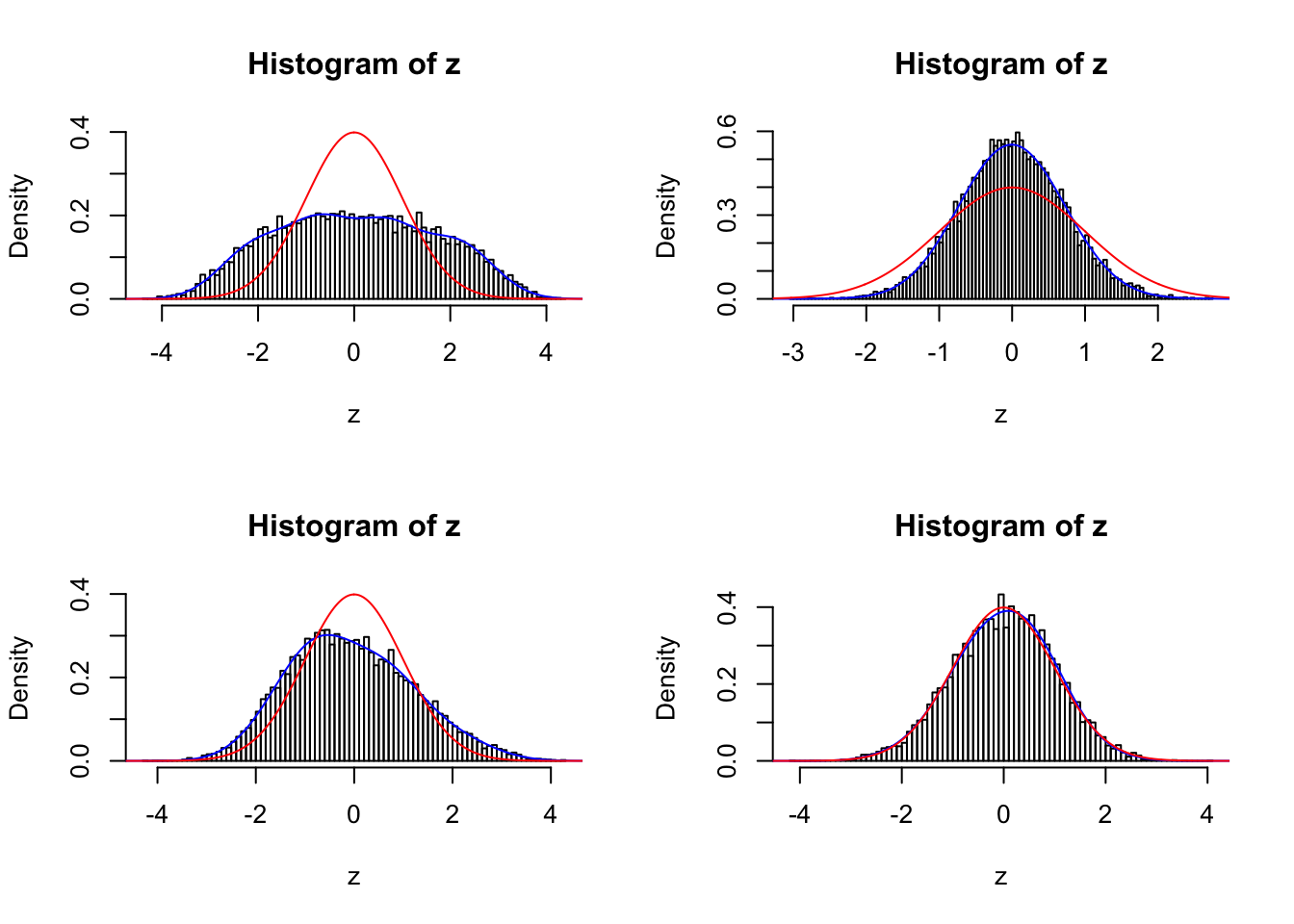
sel <- c(834, 211, 397, 748)
par(mfrow = c(2, 2))
for (i in seq(sel)) {
fit <- gdfit(z[[sel[i]]], 10)
plot.gdfit(z[[sel[i]]], fit$w, fit$L, legend = FALSE)
}
Expand here to see past versions of unnamed-chunk-15-1.png:
| Version | Author | Date |
|---|---|---|
| adeab80 | LSun | 2018-05-06 |
set.seed(6)
par(mfrow = c(2, 3))
par(mar = c(4.5, 4.5, 2, 2))
hist(pnorm(-abs(z[[834]])) * 2, prob = TRUE, xlab = "", breaks = 100, main = "(a): Histogram of two-sided p-values")
lines(c(0, 1), c(1, 1), col = "red")
hist(z[[834]], prob = TRUE, breaks = 100, xlab = "", xlim = c(-4.5, -2), main = "(b): Left tail of correlated z-scores")
lines(seq(-6, 6, by = 0.01), dnorm(seq(-6, 6, by = 0.01), 0, sd(z[[834]])), col = "blue")
lines(seq(-6, 6, by = 0.01), dnorm(seq(-6, 6, by = 0.01)), col = "red")
hist(z[[834]], prob = TRUE, breaks = 100, xlab = "", xlim = c(2, 4.5), main = "(c): Right tail of correlated z-scores")
lines(seq(-6, 6, by = 0.01), dnorm(seq(-6, 6, by = 0.01)), col = "red")
p <- pnorm(-abs(z[[834]])) * 2
plot(sample(-log(pnorm(-abs(z[[834]])) * 2)), ylim = c(0, 20), ylab = "-log(p)", main = expression(paste("(d): Correlated ", N(0, 1))))
abline(h = -log(0.005), col = "red")
abline(h = -log(pnorm(-sqrt(2 * log(1e4))) * 2), col = "blue")
abline(h = -log(0.05 / 1e4), col = "green")
plot(-log(pnorm(-abs(rnorm(1e4))) * 2), ylim = c(0, 20), ylab = "-log(p)", main = expression(paste("(e): Independent ", N(0, 1))))
abline(h = -log(0.005), col = "red")
abline(h = -log(pnorm(-sqrt(2 * log(1e4))) * 2), col = "blue")
abline(h = -log(0.05 / 1e4), col = "green")
plot(-log(pnorm(-abs(rnorm(1e4, 0, 1.6))) * 2), ylim = c(0, 20), ylab = "-log(p)", main = expression(paste("(f): Independent ", N(0, 1.6^2))))
abline(h = -log(0.005), col = "red")
abline(h = -log(pnorm(-sqrt(2 * log(1e4))) * 2), col = "blue")
abline(h = -log(0.05 / 1e4), col = "green")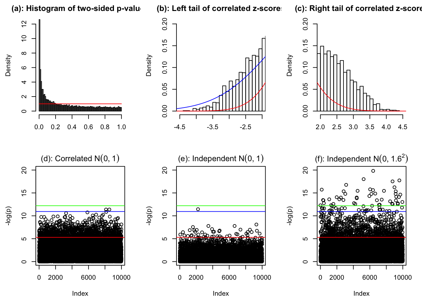
Expand here to see past versions of unnamed-chunk-16-1.png:
| Version | Author | Date |
|---|---|---|
| adeab80 | LSun | 2018-05-06 |
p.bh <- p.adjust(p, method = "BH")
sum(p.bh <= 0.05)[1] 575plot(sort(log(p)), cex = 0.25, pch = 19, ylim = c(-19, 0), xlab = "Order", ylab = "log(p)")
set.seed(6)
z.indep <- rnorm(1e4)
points(sort(log(pnorm(-abs(z.indep)) * 2)), cex = 0.25, pch = 19, col = "blue")
z.indep <- rnorm(1e4, 0, 1.6)
points(sort(log(pnorm(-abs(z.indep)) * 2)), cex = 0.25, pch = 19, col = "green")
plot(sort(log(p)), cex = 0.25, pch = 19, ylim = c(-19, -2.5), xlim = c(1, 850), xlab = "Order", ylab = "log(p)")
set.seed(6)
z.indep <- rnorm(1e4)
points(sort(log(pnorm(-abs(z.indep)) * 2)), cex = 0.25, pch = 19, col = "blue")
z.indep <- rnorm(1e4, 0, 1.6)
points(sort(log(pnorm(-abs(z.indep)) * 2)), cex = 0.25, pch = 19, col = "green")
abline(h = log(0.005), col = "red", lty = 2)
abline(h = log(pnorm(-sqrt(2 * log(1e4))) * 2), col = "red", lty = 2)
abline(h = log(0.05 / 1e4), col = "red", lty = 2)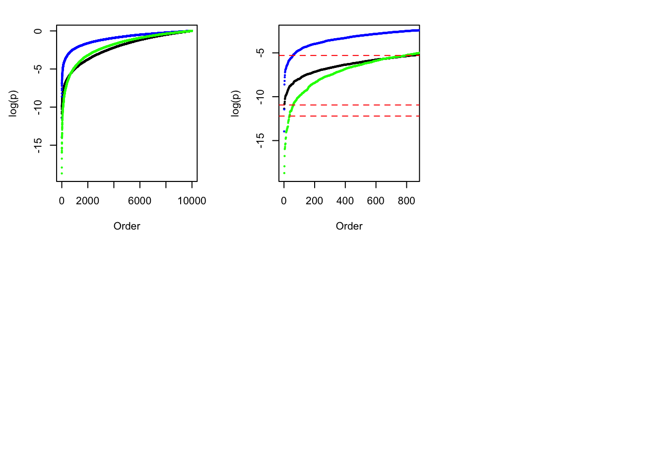
Expand here to see past versions of unnamed-chunk-16-2.png:
| Version | Author | Date |
|---|---|---|
| adeab80 | LSun | 2018-05-06 |
W.sim.gd <- sapply(Z.sim, function (z) {fit.z <- gdfit(z, L = 10); return(
list(w = fit.z$w, status = fit.z$status))})W.gtex.gd <- sapply(Z.gtex, function (z) {fit.z <- gdfit(z, L = 10); return(
list(w = fit.z$w, status = fit.z$status))})Shoulder inflation
z <- z.mat.sel[3, ]
p <- pnorm(-abs(z)) * 2
## the image is 7.5 * 3
setEPS()
postscript("../output/fig/cor_z_cdf.eps", width = 7.5, height = 3)
par(mfrow = c(1, 3))
par(oma = c(4, 2.5, 0, 0)) # make room (i.e. the 4's) for the overall x and y axis titles
par(mar = c(2, 2, 2.5, 1)) # make the plots be closer together
plot(ecdf(z), xlab = "", ylab = "", lwd = 2, main = expression("(a): CDF of All"), cex.main = 1.5)
lines(seq(-6, 6, by = 0.01), pnorm(seq(-6, 6, by = 0.01)), col = "blue", lwd = 2)
lines(seq(-6, 6, by = 0.01), pnorm(seq(-6, 6, by = 0.01), 0, 1.6), col = "green", lwd = 2)
rect(xleft = c(-5, 2.5),
xright = c(-2.5, 5),
ytop = c(0.05, 1),
ybottom = c(0, 0.95), border = "red", lty = c(1, 5))
plot(ecdf(z), xlab = "", ylab = "", main = expression("(b): Left Tail"), lwd = 2, xlim = c(-5, -2.5), ylim = c(0, 0.05), cex.main = 1.5, bty = "n")
box(col = "red")
lines(seq(-6, 6, by = 0.01), pnorm(seq(-6, 6, by = 0.01)), col = "blue", lwd = 2)
lines(seq(-6, 6, by = 0.01), pnorm(seq(-6, 6, by = 0.01), 0, 1.6), col = "green", lwd = 2)
plot(ecdf(z), xlab = "", ylab = "", main = expression("(c): Right tail"), lwd = 2, xlim = c(2.5, 5), ylim = c(0.95, 1), cex.main = 1.5, bty = "n")
box(col = "red", lty = 5)
lines(seq(-6, 6, by = 0.01), pnorm(seq(-6, 6, by = 0.01)), col = "blue", lwd = 2)
lines(seq(-6, 6, by = 0.01), pnorm(seq(-6, 6, by = 0.01), 0, 1.6), col = "green", lwd = 2)
mtext('CDF', side = 2, outer = TRUE, line = 1)
legend("bottomleft", inset = c(-1.275, -0.35), legend = c("N(0, 1)", expression(N(0, 1.6^2))), lty = 1, lwd = 2, xpd = NA, col = c("blue", "green"), ncol = 2, cex = 1.25)
dev.off()quartz_off_screen
2 # 7.5 * 3
setEPS()
postscript("../output/fig/cor_z_pval.eps", width = 7.5, height = 3.3)
par(mfrow = c(1, 3))
par(oma = c(4, 2.5, 0, 0)) # make room (i.e. the 4's) for the overall x and y axis titles
par(mar = c(4.5, 2, 2.5, 1)) # make the plots be closer together
set.seed(5)
p.norm.1 <- pnorm(-abs(rnorm(1e4))) * 2
set.seed(25)
p.norm.1.6 <- pnorm(-abs(rnorm(1e4, 0, 1.6))) * 2
y.max <- -log(min(p.norm.1, p, p.norm.1.6))
y.max <- 20
plot(sample(-log(p)), ylim = c(0, y.max), ylab = "-log(p)", main = expression(paste("(d): Correlated ", N(0, 1))), cex.main = 1.5, cex.lab = 1.5)
abline(h = -log(0.005), col = "red", lwd = 2)
abline(h = -log(pnorm(-sqrt(2 * log(1e4))) * 2), col = "orange", lwd = 2)
abline(h = -log(0.05 / 1e4), col = "yellow", lwd = 2)
plot(-log(p.norm.1), ylim = c(0, y.max), ylab = "-log(p)", main = expression(paste("(e): Independent ", N(0, 1))), col = "blue", cex.main = 1.5, cex.lab = 1.5)
abline(h = -log(0.005), col = "red", lwd = 2)
abline(h = -log(pnorm(-sqrt(2 * log(1e4))) * 2), col = "orange", lwd = 2)
abline(h = -log(0.05 / 1e4), col = "yellow", lwd = 2)
plot(-log(p.norm.1.6), ylim = c(0, y.max), ylab = "-log(p)", main = expression(paste("(f): Independent ", N(0, 1.6^2))), col = "green", cex.main = 1.5, cex.lab = 1.5)
abline(h = -log(0.005), col = "red", lwd = 2)
abline(h = -log(pnorm(-sqrt(2 * log(1e4))) * 2), col = "orange", lwd = 2)
abline(h = -log(0.05 / 1e4), col = "yellow", lwd = 2)
mtext('-log(p)', side = 2, outer = TRUE, line = 1)
legend("bottomleft", inset = c(-2.01, -0.51), legend = c("0.005", "Universal Threshold", "Bonferroni"), lty = 1, lwd = 2, xpd = NA, col = c("red", "orange", "yellow"), ncol = 3, cex = 1.25)
dev.off()quartz_off_screen
2 ## under 0.005
sum(p <= 0.005)[1] 809p.bh <- p.adjust(p, method = "BH")
## BHq at FDR 0.05
sum(p.bh <= 0.05)[1] 506fit.q <- qvalue::qvalue(p)
## pi0 by qvalue
1 - fit.q$pi0[1] 0.566462## qvalue at FDR 0.05
sum(fit.q$qvalues <= 0.05)[1] 2162## pi0 by ashr
fit.a <- ashr::ash(z, 1, method = "fdr")
1 - ashr::get_pi0(fit.a)[1] 0.98599## ashr at FDR 0.05
sum(ashr::get_qvalue(fit.a) <= 0.05)[1] 10000Deconvolution
KFE <- function(y, T = 300, lambda = 1/3){
# Kernel Fourier Estimator: Stefanski and Carroll (Statistics, 1990)
ks <- function(s,x) exp(s^2/2) * cos(s * x)
K <- function(t, y, lambda = 1/3){
k <- y
for(i in 1:length(y)){
k[i] <- integrate(ks, 0, 1/lambda, x = (y[i] - t))$value/pi
}
mean(k)
}
eps <- 1e-04
if(length(T) == 1) T <- seq(min(y)-eps, max(y)+eps, length = T)
g <- T
for(j in 1:length(T))
g[j] <- K(T[j], y, lambda = lambda)
list(x = T, y = g)
}
biweight <- function(x0, x, bw){
t <- (x - x0)/bw
(1-t^2)^2*((t> -1 & t<1)-0) *15/16
}
CDF.KW <- function(h, interp = FALSE, eps = 0.001, bw = 0.7){
#Wasserstein distance: ||G-H||_W
if(interp == "biweight"){
yk = h$x
for (j in 1:length(yk))
yk[j] = sum(biweight(h$x[j], h$x, bw = bw)*h$y/sum(h$y))
H <- cumsum(yk)
H <- H/H[length(H)]
}
else {
H <- cumsum(h$y)
H <- H/H[length(H)]
}
return(H)
}
library(deconvolveR)G <- function (t) {
0.6 * pnorm(t, 0, 0) + 0.3 * pnorm(t, 0, 1) + 0.1 * pnorm(t, 0, 3)
}
set.seed(777)
theta <- sample(c(
rnorm(6e3, 0, 0),
rnorm(3e3, 0, 1),
rnorm(1e3, 0, 3)
))set.seed(777)
r <- readRDS("../data/liver.rds")
nsamp <- 5
ngene <- 1e4
Y = lcpm(r)
subset = top_genes_index(ngene, Y)
r = r[subset,]
counts <- r[, sample(ncol(r), 2 * nsamp)]
design <- model.matrix(~c(rep(0, nsamp), rep(1, nsamp)))
summary <- count_to_summary(counts, design)
s <- summary$sebetahat
s <- s / sqrt(mean(s^2))x.plot <- seq(-6, 6, by = 0.01)
G.plot <- G(x.plot)
for (i in 3 : 5) {
if (i != 5) {
z <- z.mat.sel[i, ]
} else {
z <- rnorm(1e4)
}
X <- theta + s * z
Z <- theta + z
## Truth
True.data <- cbind.data.frame(
Method = "True",
x = x.plot,
cdfhat = G.plot
)
## ASH
fit.ash <- ashr::ash(X, s, method = "fdr", mixcompdist = "normal")
ash.plot <- as.numeric(ashr::mixcdf(ashr::get_fitted_g(fit.ash), x.plot))
ASH.data <- cbind.data.frame(
Method = "ASH",
x = x.plot,
cdfhat = ash.plot
)
## CASH
fit.cash <- gdash(X, s)
cash.plot <- as.numeric(ashr::mixcdf(ashr::get_fitted_g(fit.cash), x.plot))
CASH.data <- cbind.data.frame(
Method = "CASH",
x = x.plot,
cdfhat = cash.plot
)
## Efron's BD (2016)
fit.bd <- deconvolveR::deconv(tau = x.plot, X = Z, family = "Normal", deltaAt = 0)
BD.data <- cbind.data.frame(
Method = "Efron",
x = fit.bd$stats[, 1],
cdfhat = fit.bd$stats[, 4]
)
## Kiefer-Wolfowitz's NPMLE (1956)
## implemented by Koenker-Mizera-Gu's REBayes (2016)
v = seq(-6, 6, by = 0.01)
fit.kw <- REBayes::GLmix(x = X, v = v, sigma = s)
kw.plot <- CDF.KW(fit.kw)
KW.data <- cbind.data.frame(
Method = "KW",
x = fit.kw$x,
cdfhat = kw.plot
)
## KW smoothed by the biweight kernel
kws.plot <- CDF.KW(fit.kw, interp = "biweight")
KWs.data <- cbind.data.frame(
Method = "KWs",
x = fit.kw$x,
cdfhat = kws.plot
)
## kernal deconvolution by Stefanski and Carroll 1990
## implemented by `decon`
fit.fk <- decon::DeconCdf(y = X, sig = s, error = "normal")
FK.data <- cbind.data.frame(
Method = "Fourier-Kernel",
x = fit.fk$x,
cdfhat = fit.fk$y
)
if (i == 3) {
deconv.inf.ggdata <- cbind.data.frame(
Noise = "Inflated Noise",
rbind.data.frame(
True.data,
KW.data,
BD.data,
ASH.data,
CASH.data
)
)
} else if (i == 4) {
deconv.def.ggdata <- cbind.data.frame(
Noise = "Deflated Noise",
rbind.data.frame(
True.data,
KW.data,
BD.data,
ASH.data,
CASH.data
)
)
} else {
deconv.ind.ggdata <- cbind.data.frame(
Noise = "Independent Noise",
rbind.data.frame(
True.data,
KW.data,
BD.data,
ASH.data,
CASH.data
)
)
}
}Warning in REBayes::KWDual(A, rep(1, k), normalize(w), control = control): estimated mixing distribution has some negative values:
consider reducing rtol
Warning in REBayes::KWDual(A, rep(1, k), normalize(w), control = control): estimated mixing distribution has some negative values:
consider reducing rtol
Warning in REBayes::KWDual(A, rep(1, k), normalize(w), control = control): estimated mixing distribution has some negative values:
consider reducing rtol
Warning in REBayes::KWDual(A, rep(1, k), normalize(w), control = control): estimated mixing distribution has some negative values:
consider reducing rtol
Warning in REBayes::KWDual(A, rep(1, k), normalize(w), control = control): estimated mixing distribution has some negative values:
consider reducing rtol
Warning in REBayes::KWDual(A, rep(1, k), normalize(w), control = control): estimated mixing distribution has some negative values:
consider reducing rtolWarning in stats::nlm(f = loglik, p = aStart, gradtol = 1e-10, ...): NA/Inf
replaced by maximum positive value
Warning in stats::nlm(f = loglik, p = aStart, gradtol = 1e-10, ...): NA/Inf
replaced by maximum positive valueWarning in REBayes::KWDual(A, rep(1, k), normalize(w), control = control): estimated mixing distribution has some negative values:
consider reducing rtol
Warning in REBayes::KWDual(A, rep(1, k), normalize(w), control = control): estimated mixing distribution has some negative values:
               consider reducing rtol

Warning in REBayes::KWDual(A, rep(1, k), normalize(w), control = control): estimated mixing distribution has some negative values:
               consider reducing rtol

Warning in REBayes::KWDual(A, rep(1, k), normalize(w), control = control): estimated mixing distribution has some negative values:
               consider reducing rtol

Warning in REBayes::KWDual(A, rep(1, k), normalize(w), control = control): estimated mixing distribution has some negative values:
               consider reducing rtol

Warning in REBayes::KWDual(A, rep(1, k), normalize(w), control = control): estimated mixing distribution has some negative values:
               consider reducing rtol

Warning in REBayes::KWDual(A, rep(1, k), normalize(w), control = control): estimated mixing distribution has some negative values:
               consider reducing rtol
Warning in REBayes::KWDual(A, rep(1, k), normalize(w), control = control): estimated mixing distribution has some negative values:
consider reducing rtol
Warning in REBayes::KWDual(A, rep(1, k), normalize(w), control = control): estimated mixing distribution has some negative values:
consider reducing rtol
Warning in REBayes::KWDual(A, rep(1, k), normalize(w), control = control): estimated mixing distribution has some negative values:
consider reducing rtol
Warning in REBayes::KWDual(A, rep(1, k), normalize(w), control = control): estimated mixing distribution has some negative values:
consider reducing rtol
Warning in REBayes::KWDual(A, rep(1, k), normalize(w), control = control): estimated mixing distribution has some negative values:
consider reducing rtol
Warning in REBayes::KWDual(A, rep(1, k), normalize(w), control = control): estimated mixing distribution has some negative values:
consider reducing rtolWarning in stats::nlm(f = loglik, p = aStart, gradtol = 1e-10, ...): NA/Inf
replaced by maximum positive value
Warning in stats::nlm(f = loglik, p = aStart, gradtol = 1e-10, ...): NA/Inf
replaced by maximum positive value

Warning in stats::nlm(f = loglik, p = aStart, gradtol = 1e-10, ...): NA/Inf
replaced by maximum positive value
Warning in stats::nlm(f = loglik, p = aStart, gradtol = 1e-10, ...): NA/Inf
replaced by maximum positive value
Warning in stats::nlm(f = loglik, p = aStart, gradtol = 1e-10, ...): NA/Inf
replaced by maximum positive valuedeconv.ggdata <- rbind.data.frame(
deconv.def.ggdata,
deconv.ind.ggdata,
deconv.inf.ggdata
)method.name <- c("True", "KW NPMLE", "Efron g-modeling", "ASH", "CASH")
method.col <- scales::hue_pal()(5)
method.linetype <- c("longdash", rep("solid", 4))## plotting
ggplot(data = deconv.ggdata, aes(x = x, y = cdfhat, col = Method, linetype = Method)) +
geom_line() +
facet_wrap(~Noise, nrow = 1) +
xlim(-5, 5) +
scale_linetype_manual(values = method.linetype, labels = method.name, guide = guide_legend(nrow = 1)) +
scale_color_manual(values = method.col, labels = method.name, guide = guide_legend(nrow = 1)) +
labs(x = expression(theta), y = "Estimated CDF of g", title = expression(g == 0.6~delta[0] + 0.3~N(0, 1) + 0.1~N(0, 3^2))) +
theme(plot.title = element_text(size = 15, hjust = 0.5),
axis.title.x = element_text(size = 15),
axis.text.x = element_text(size = 10),
axis.title.y = element_text(size = 15),
axis.text.y = element_text(size = 10),
strip.text = element_text(size = 15),
legend.position = "bottom",
legend.title = element_blank(),
legend.background = element_rect(color = "grey"),
legend.text = element_text(size = 12)) +
ggsave("../output/fig/deconv.eps", height = 4, width = 9)Warning: Removed 1000 rows containing missing values (geom_path).
Warning: Removed 1000 rows containing missing values (geom_path).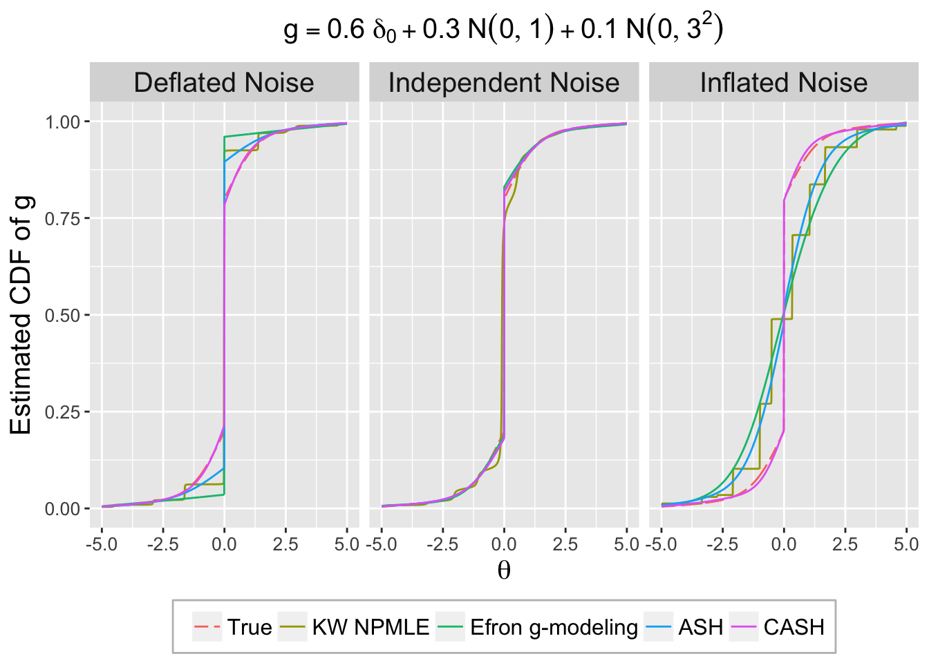
Randomization by permutating labels on GTEx data
r <- readRDS("../data/liver.rds")
ngene <- 1e4
Y = lcpm(r)
subset = top_genes_index(ngene, Y)
r = r[subset,]set.seed(777)
nsim <- 1e4
Z.list <- list()
for (i in seq(nsim)) {
## generate data
counts <- r[, sample(ncol(r))]
design <- model.matrix(~c(rep(0, 60), rep(1, 59)))
summary <- count_to_summary(counts, design)
Z <- summary$z
Z.list[[i]] <- Z
}
z.mat <- matrix(unlist(Z.list), byrow = TRUE, nrow = nsim)png("../output/fig/ecdf_by_dataset.png", width = 5, height = 5, units = "in", res = 600)
par(mar = c(4.5, 4.5, 1, 1))
plot(0, type = "n", xlim = c(-5, 5), ylim = c(0, 1), ylab = "(Empirical) CDF", xlab = "z", cex.lab = 2)
for (i in seq(nrow(z.mat))) {
lines(ecdf(z.mat[i, ]), lwd = 1, col = "grey75")
}
lines(seq(-6, 6, by = 0.01), pnorm(seq(-6, 6, by = 0.01)), lwd = 2, col = "blue")
legend("bottomright", lwd = 1 : 2, col = c("grey75", "blue"), c(expression("F"[n]), expression(Phi)), bty = "n")
dev.off()quartz_off_screen
2 png("../output/fig/ecdf_by_gene.png", width = 5, height = 5, units = "in", res = 600)
par(mar = c(4.5, 4.5, 1, 1))
plot(0, type = "n", xlim = c(-5, 5), ylim = c(0, 1), ylab = "(Empirical) CDF", xlab = "z", cex.lab = 2)
for (i in seq(ncol(z.mat))) {
lines(ecdf(z.mat[, i]), lwd = 1, col = "grey75")
}
lines(seq(-6, 6, by = 0.01), pnorm(seq(-6, 6, by = 0.01)), lwd = 2, col = "blue")
legend("bottomright", lwd = 1 : 2, col = c("grey75", "blue"), c(expression("F"[n]), expression(Phi)), bty = "n")
dev.off()quartz_off_screen
2 png("../output/fig/ecdf_ind.png", width = 5, height = 5, units = "in", res = 600)
par(mar = c(4.5, 4.5, 1, 1))
plot(0, type = "n", xlim = c(-5, 5), ylim = c(0, 1), ylab = "(Empirical) CDF", xlab = "z", cex.lab = 2)
for (i in seq(ncol(z.mat))) {
lines(ecdf(rnorm(nrow(z.mat))), lwd = 1, col = "grey75")
}
lines(seq(-6, 6, by = 0.01), pnorm(seq(-6, 6, by = 0.01)), lwd = 2, col = "blue")
legend("bottomright", lwd = 1 : 2, col = c("grey75", "blue"), c(expression("F"[n]), expression(Phi)), bty = "n")
dev.off()quartz_off_screen
2 Random by each gene
r <- readRDS("../data/liver.rds")
ngene <- 1e4
Y = lcpm(r)
subset = top_genes_index(ngene, Y)
r = r[subset,]nsamp <- 5set.seed(777)
nsim <- 1e4
Z.list <- list()
for (i in seq(nsim)) {
## generate data
counts <- t(apply(r, 1, sample, 2 * nsamp))
design <- model.matrix(~c(rep(0, nsamp), rep(1, nsamp)))
summary <- count_to_summary(counts, design)
Z <- summary$z
Z.list[[i]] <- Z
}
z.mat.rand.each.gene <- matrix(unlist(Z.list), byrow = TRUE, nrow = nsim)png("../output/fig/ecdf_cor_rand_gene.png", width = 5, height = 5, units = "in", res = 600)
par(mar = c(4.5, 4.5, 1, 1))
plot(0, type = "n", xlim = c(-5, 5), ylim = c(0, 1), ylab = "(Empirical) CDF", xlab = "z", cex.lab = 2)
for (i in seq(nrow(z.mat.rand.each.gene))) {
lines(ecdf(z.mat.rand.each.gene[i, ]), lwd = 1, col = "grey75")
}
lines(seq(-6, 6, by = 0.01), pnorm(seq(-6, 6, by = 0.01)), lwd = 2, col = "blue")
legend("bottomright", lwd = 1 : 2, col = c("grey75", "blue"), c(expression("F"[n]), expression(Phi)), bty = "n")
dev.off()quartz_off_screen
2 Session information
sessionInfo()R version 3.4.3 (2017-11-30)
Platform: x86_64-apple-darwin15.6.0 (64-bit)
Running under: macOS High Sierra 10.13.5
Matrix products: default
BLAS: /Library/Frameworks/R.framework/Versions/3.4/Resources/lib/libRblas.0.dylib
LAPACK: /Library/Frameworks/R.framework/Versions/3.4/Resources/lib/libRlapack.dylib
locale:
[1] en_US.UTF-8/en_US.UTF-8/en_US.UTF-8/C/en_US.UTF-8/en_US.UTF-8
attached base packages:
[1] stats graphics grDevices utils datasets methods base
other attached packages:
[1] polynom_1.3-9 deconvolveR_1.1 decon_1.2-4
[4] reshape2_1.4.3 ggplot2_2.2.1 plyr_1.8.4
[7] edgeR_3.20.9 limma_3.34.9 ashr_2.2-7
[10] Rmosek_8.0.69 PolynomF_1.0-2 CVXR_0.95
[13] REBayes_1.3 Matrix_1.2-14 SQUAREM_2017.10-1
[16] EQL_1.0-0 ttutils_1.0-1
loaded via a namespace (and not attached):
[1] qvalue_2.10.0 locfit_1.5-9.1 splines_3.4.3
[4] lattice_0.20-35 colorspace_1.3-2 htmltools_0.3.6
[7] yaml_2.1.19 gmp_0.5-13.1 rlang_0.2.0
[10] R.oo_1.22.0 pillar_1.2.2 Rmpfr_0.7-0
[13] R.utils_2.6.0 bit64_0.9-7 scs_1.1-1
[16] foreach_1.4.4 stringr_1.3.1 munsell_0.4.3
[19] gtable_0.2.0 workflowr_1.0.1 R.methodsS3_1.7.1
[22] codetools_0.2-15 evaluate_0.10.1 labeling_0.3
[25] knitr_1.20 doParallel_1.0.11 pscl_1.5.2
[28] parallel_3.4.3 Rcpp_0.12.16 backports_1.1.2
[31] scales_0.5.0 truncnorm_1.0-8 bit_1.1-13
[34] digest_0.6.15 stringi_1.2.2 grid_3.4.3
[37] rprojroot_1.3-2 ECOSolveR_0.4 tools_3.4.3
[40] magrittr_1.5 lazyeval_0.2.1 tibble_1.4.2
[43] whisker_0.3-2 MASS_7.3-50 assertthat_0.2.0
[46] rmarkdown_1.9 iterators_1.0.9 R6_2.2.2
[49] git2r_0.21.0 compiler_3.4.3 This reproducible R Markdown analysis was created with workflowr 1.0.1