FWER Procedures on Simulated Correlated Null
Lei Sun
2016-11-29
Last updated: 2018-05-12
workflowr checks: (Click a bullet for more information)-
✔ R Markdown file: up-to-date
Great! Since the R Markdown file has been committed to the Git repository, you know the exact version of the code that produced these results.
-
✔ Environment: empty
Great job! The global environment was empty. Objects defined in the global environment can affect the analysis in your R Markdown file in unknown ways. For reproduciblity it’s best to always run the code in an empty environment.
-
✔ Seed:
set.seed(12345)The command
set.seed(12345)was run prior to running the code in the R Markdown file. Setting a seed ensures that any results that rely on randomness, e.g. subsampling or permutations, are reproducible. -
✔ Session information: recorded
Great job! Recording the operating system, R version, and package versions is critical for reproducibility.
-
Great! You are using Git for version control. Tracking code development and connecting the code version to the results is critical for reproducibility. The version displayed above was the version of the Git repository at the time these results were generated.✔ Repository version: 140be7f
Note that you need to be careful to ensure that all relevant files for the analysis have been committed to Git prior to generating the results (you can usewflow_publishorwflow_git_commit). workflowr only checks the R Markdown file, but you know if there are other scripts or data files that it depends on. Below is the status of the Git repository when the results were generated:
Note that any generated files, e.g. HTML, png, CSS, etc., are not included in this status report because it is ok for generated content to have uncommitted changes.Ignored files: Ignored: .DS_Store Ignored: .Rhistory Ignored: .Rproj.user/ Ignored: analysis/.DS_Store Ignored: analysis/BH_robustness_cache/ Ignored: analysis/FDR_Null_cache/ Ignored: analysis/FDR_null_betahat_cache/ Ignored: analysis/Rmosek_cache/ Ignored: analysis/StepDown_cache/ Ignored: analysis/alternative2_cache/ Ignored: analysis/alternative_cache/ Ignored: analysis/ash_gd_cache/ Ignored: analysis/average_cor_gtex_2_cache/ Ignored: analysis/average_cor_gtex_cache/ Ignored: analysis/brca_cache/ Ignored: analysis/cash_deconv_cache/ Ignored: analysis/cash_fdr_1_cache/ Ignored: analysis/cash_fdr_2_cache/ Ignored: analysis/cash_fdr_3_cache/ Ignored: analysis/cash_fdr_4_cache/ Ignored: analysis/cash_fdr_5_cache/ Ignored: analysis/cash_fdr_6_cache/ Ignored: analysis/cash_plots_cache/ Ignored: analysis/cash_sim_1_cache/ Ignored: analysis/cash_sim_2_cache/ Ignored: analysis/cash_sim_3_cache/ Ignored: analysis/cash_sim_4_cache/ Ignored: analysis/cash_sim_5_cache/ Ignored: analysis/cash_sim_6_cache/ Ignored: analysis/cash_sim_7_cache/ Ignored: analysis/correlated_z_2_cache/ Ignored: analysis/correlated_z_3_cache/ Ignored: analysis/correlated_z_cache/ Ignored: analysis/create_null_cache/ Ignored: analysis/cutoff_null_cache/ Ignored: analysis/design_matrix_2_cache/ Ignored: analysis/design_matrix_cache/ Ignored: analysis/diagnostic_ash_cache/ Ignored: analysis/diagnostic_correlated_z_2_cache/ Ignored: analysis/diagnostic_correlated_z_3_cache/ Ignored: analysis/diagnostic_correlated_z_cache/ Ignored: analysis/diagnostic_plot_2_cache/ Ignored: analysis/diagnostic_plot_cache/ Ignored: analysis/efron_leukemia_cache/ Ignored: analysis/fitting_normal_cache/ Ignored: analysis/gaussian_derivatives_2_cache/ Ignored: analysis/gaussian_derivatives_3_cache/ Ignored: analysis/gaussian_derivatives_4_cache/ Ignored: analysis/gaussian_derivatives_5_cache/ Ignored: analysis/gaussian_derivatives_cache/ Ignored: analysis/gd-ash_cache/ Ignored: analysis/gd_delta_cache/ Ignored: analysis/gd_lik_2_cache/ Ignored: analysis/gd_lik_cache/ Ignored: analysis/gd_w_cache/ Ignored: analysis/knockoff_10_cache/ Ignored: analysis/knockoff_2_cache/ Ignored: analysis/knockoff_3_cache/ Ignored: analysis/knockoff_4_cache/ Ignored: analysis/knockoff_5_cache/ Ignored: analysis/knockoff_6_cache/ Ignored: analysis/knockoff_7_cache/ Ignored: analysis/knockoff_8_cache/ Ignored: analysis/knockoff_9_cache/ Ignored: analysis/knockoff_cache/ Ignored: analysis/knockoff_var_cache/ Ignored: analysis/marginal_z_alternative_cache/ Ignored: analysis/marginal_z_cache/ Ignored: analysis/mosek_reg_2_cache/ Ignored: analysis/mosek_reg_4_cache/ Ignored: analysis/mosek_reg_5_cache/ Ignored: analysis/mosek_reg_6_cache/ Ignored: analysis/mosek_reg_cache/ Ignored: analysis/pihat0_null_cache/ Ignored: analysis/plot_diagnostic_cache/ Ignored: analysis/poster_obayes17_cache/ Ignored: analysis/real_data_simulation_2_cache/ Ignored: analysis/real_data_simulation_3_cache/ Ignored: analysis/real_data_simulation_4_cache/ Ignored: analysis/real_data_simulation_5_cache/ Ignored: analysis/real_data_simulation_cache/ Ignored: analysis/rmosek_primal_dual_2_cache/ Ignored: analysis/rmosek_primal_dual_cache/ Ignored: analysis/seqgendiff_cache/ Ignored: analysis/simulated_correlated_null_2_cache/ Ignored: analysis/simulated_correlated_null_3_cache/ Ignored: analysis/simulated_correlated_null_cache/ Ignored: analysis/simulation_real_se_2_cache/ Ignored: analysis/simulation_real_se_cache/ Ignored: analysis/smemo_2_cache/ Ignored: data/LSI/ Ignored: docs/.DS_Store Ignored: docs/figure/.DS_Store Ignored: output/fig/ Untracked files: Untracked: docs/figure/smemo.rmd/ Unstaged changes: Modified: analysis/smemo.rmd
Expand here to see past versions:
| File | Version | Author | Date | Message |
|---|---|---|---|---|
| Rmd | cc0ab83 | Lei Sun | 2018-05-11 | update |
| html | 0f36d99 | LSun | 2017-12-21 | Build site. |
| html | 853a484 | LSun | 2017-11-07 | Build site. |
| html | 1ea081a | LSun | 2017-07-03 | sites |
| html | 7693edf | LSun | 2017-02-14 | pipeline |
| Rmd | 681085c | LSun | 2017-02-10 | fdr |
| html | 681085c | LSun | 2017-02-10 | fdr |
| html | 81d84f5 | LSun | 2017-02-10 | FDR |
| Rmd | 2696cb2 | LSun | 2017-02-10 | fwer |
| html | 2696cb2 | LSun | 2017-02-10 | fwer |
| html | 066c544 | LSun | 2017-02-03 | StepDown |
| Rmd | 4afbe4e | LSun | 2017-02-03 | StepDown |
| html | 59fd661 | LSun | 2017-02-03 | Build site. |
| Rmd | c4165dc | LSun | 2017-02-03 | simulation |
| html | c4165dc | LSun | 2017-02-03 | simulation |
| Rmd | 313897f | LSun | 2017-02-03 | details |
| html | 313897f | LSun | 2017-02-03 | details |
| html | 36c1e4c | LSun | 2017-02-03 | Build site. |
| Rmd | d25a6e3 | LSun | 2017-02-03 | step-down |
| html | d25a6e3 | LSun | 2017-02-03 | step-down |
Last updated: 2018-05-12
Code version: 140be7f
Introduction
In order to understand the behavior of \(p\)-values of top expressed, correlated genes under the global null, simulated from GTEx data, we apply two FWER-controlling multiple comparison procedures, Holm’s “step-down” (Holm 1979) and Hochberg’s “step-up.” (Hochberg 1988)
Holm’s step-down procedure: start from the smallest \(p\)-value
It can be shown that Holm’s procedure conservatively controls the FWER in the strong sense, under arbitrary correlation among \(p\)-values.
First, order the \(p\)-values
\[ p_{(1)} \leq p_{(2)} \leq \cdots \leq p_{(n)} \]
and let \(H_{(1)}, H_{(2)}, \ldots, H_{(n)}\) be the corresponding hypotheses. Then examine the \(p\)-values in order.
Step 1: If \(p_{(1)} \leq \alpha/n\) reject \(H_{(1)}\) and go to Step 2. Otherwise, accept \(H_{(1)}, H_{(2)}, \ldots, H_{(n)}\) and stop.
……
Step \(i\): If \(p_{(i)} \leq \alpha / (n − i + 1)\) reject \(H_{(i)}\) and go to step \(i + 1\). Otherwise, accept \(H_{(i)}, H_{(i + 1)}, \ldots, H_{(n)}\) and stop.
……
Step \(n\): If \(p_{(n)} \leq \alpha\), reject \(H_{(n)}\). Otherwise, accept \(H_{(n)}\).
Hence the procedure starts with the most extreme (smallest) \(p\)-value and stops the first time \(p_{(i)}\) exceeds the critical value \(\alpha_i = \alpha/(n − i + 1)\).
It can be shown that Holm’s procedure conservatively controls the FWER in the strong sense, under arbitrary correlation among \(p\)-values.
Hochberg’s step-up procedure: start from the largest \(p\)-value
It can be shown that Hochberg’s procedure conservatively controls the FWER in the strong sense, when \(p\)-values are independent.
First, order the \(p\)-values
\[ p_{(1)} \leq p_{(2)} \leq \cdots \leq p_{(n)} \]
and let \(H_{(1)}, H_{(2)}, \ldots, H_{(n)}\) be the corresponding hypotheses. Then examine the \(p\)-values in order.
Step 1: If \(p_{(n)} \leq \alpha\) reject \(H_{(1)}, \ldots, H_{(n)}\) and stop. Otherwise, accept \(H_{(n)}\) and go to step 2.
……
Step \(i\): If \(p_{(n - i + 1)} \leq \alpha / i\) reject \(H_{(1)}, \ldots, H_{(n - i + 1)}\) and stop. Otherwise, accept \(H_{(n - i + 1)}\) and go to step \(i + 1\).
……
Step \(n\): If \(p_{(1)} \leq \alpha / n\), reject \(H_{(1)}\). Otherwise, accept \(H_{(1)}\).
Hence the procedure starts with the least extreme (largest) \(p\)-value and stops the first time \(p_{(i)}\) falls below the critical value \(\alpha_i = \alpha/(n − i + 1)\).
It can be shown that Hochberg’s procedure conservatively controls the FWER in the strong sense, when \(p\)-values are independent.
Sarkar 1998 also pointed out that Hochberg’s procedure can control the FWER strongly under certain dependency among the test statistics, such as a multivariate normal with a common marginal distribution and positive correlations.
Holm’s procedure is based on Bonferroni correction, whereas Hochberg’s on Sime’s inequality. Both use exactly the same thresholds, comparing \(p_{(i)}\) with \(\alpha/(n − i + 1)\), yet Holm’s starts from the smallest \(p\)-value, and Hochberg’s from the largest. Hochberg’s is thus strictly more powerful than Holm’s.
Result
Now we apply the two procedures to the simulated, correlated null data.
p1 = read.table("../output/p_null_liver.txt")
p2 = read.table("../output/p_null_liver_777.txt")
p = rbind(p1, p2)
m = nrow(p)
holm = hochberg = matrix(nrow = m, ncol = ncol(p))

for(i in 1:m){
  holm[i, ] = p.adjust(p[i, ], method = "holm") # p-values adjusted by Holm (1979)
  hochberg[i, ] = p.adjust(p[i, ], method = "hochberg") # p_values adjusted by Hochberg (1988)
}
## calculate empirical FWER at 100 nominal FWER's
alpha = seq(0, 0.15, length = 100)
fwer_holm = fwer_hochberg = c()
for (i in 1:length(alpha)) {
fwer_holm[i] = mean(apply(holm, 1, function(x) {min(x) <= alpha[i]}))
fwer_hochberg[i] = mean(apply(hochberg, 1, function(x) {min(x) <= alpha[i]}))
}
fwer_holm_se = sqrt(fwer_holm * (1 - fwer_holm) / m)
fwer_hochberg_se = sqrt(fwer_hochberg * (1 - fwer_hochberg) / m)Here at each nominal FWER from \(0\) to \(0.15\), we plot the empirical FWER, calculated from \(m = 2000\) independent simulation trials. Dotted lines indicate one standard error computed from binomial model \(= \sqrt{\hat{\text{FWER}}(1 - \hat{\text{FWER}}) / m}\).
plot(alpha, fwer_holm, pch = 1, xlab = "nominal FWER", ylab = "empirical FWER", xlim = c(0, max(alpha)), ylim = c(0, max(alpha)), cex = 0.75)
points(alpha, fwer_hochberg, col = "blue", pch = 19, cex = 0.25)
lines(alpha, fwer_holm - fwer_holm_se, lty = 3)
lines(alpha, fwer_holm + fwer_holm_se, lty = 3)
lines(alpha, fwer_hochberg + fwer_hochberg_se, lty = 3, col = "blue")
lines(alpha, fwer_hochberg - fwer_hochberg_se, lty = 3, col = "blue")

abline(0, 1, lty = 3, col = "red")
legend("topleft", c("Holm", "Hochberg"), col = c(1, "blue"), pch = c(1, 19))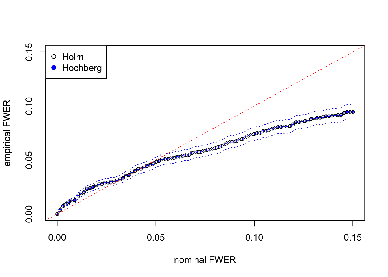
Expand here to see past versions of unnamed-chunk-3-1.png:
| Version | Author | Date |
|---|---|---|
| 0f36d99 | LSun | 2017-12-21 |
| 2696cb2 | LSun | 2017-02-10 |
The results from Holm’s step-down and Hochberg’s step-up are almost the same for this simulated data set. They both give almost the same discoveries, although in theory Hochberg’s should be strictly more powerful than Holm’s. The agreement of both procedures may indicate that test statistics are indeed inflated for moderate observations but not extreme observations.
Session Information
Session information
sessionInfo()R version 3.4.3 (2017-11-30)
Platform: x86_64-apple-darwin15.6.0 (64-bit)
Running under: macOS High Sierra 10.13.4
Matrix products: default
BLAS: /Library/Frameworks/R.framework/Versions/3.4/Resources/lib/libRblas.0.dylib
LAPACK: /Library/Frameworks/R.framework/Versions/3.4/Resources/lib/libRlapack.dylib
locale:
[1] en_US.UTF-8/en_US.UTF-8/en_US.UTF-8/C/en_US.UTF-8/en_US.UTF-8
attached base packages:
[1] stats graphics grDevices utils datasets methods base
loaded via a namespace (and not attached):
[1] workflowr_1.0.1 Rcpp_0.12.16 digest_0.6.15
[4] rprojroot_1.3-2 R.methodsS3_1.7.1 backports_1.1.2
[7] git2r_0.21.0 magrittr_1.5 evaluate_0.10.1
[10] stringi_1.1.6 whisker_0.3-2 R.oo_1.21.0
[13] R.utils_2.6.0 rmarkdown_1.9 tools_3.4.3
[16] stringr_1.3.0 yaml_2.1.18 compiler_3.4.3
[19] htmltools_0.3.6 knitr_1.20
This reproducible R Markdown analysis was created with workflowr 1.0.1