Marginal Distribution of \(z\) Scores: Null
Lei Sun
2017-04-25
Last updated: 2017-12-21
Code version: 6e42447
This simulation can be seen as an enhanced version of a previous simulation.
Introduction
An assumption of using Gaussian derivatives to fit correlated null \(z\) scores is that each of these \(z\) scores should actually be null. That is, for \(n\) \(z\) scores \(z_1, \ldots, z_n\), although the correlation between \(z_i\) and \(z_j\) are not necessarily zero, the marginal distribution of \(z_i\), \(\forall i\), should be \(N\left(0, 1\right)\).
However, in practice, it’s not easy to check whether these correlated \(z\) scores are truly marginally \(N\left(0, 1\right)\). We’ve seen that their historgram could be far from normal. Further more, \(z\) scores in different data sets are distorted by different correlation structures. Therefore, we don’t have replicates here; that is, each data set is one single realization of a lot of random variables under correlation.
For our data sets in particular, let \(Z = \left[z_{ij}\right]_{m \times n}\) be the matrix of \(z\) scores. Each \(z_{ij}\) denotes the gene differential expression \(z\) score for gene \(j\) in the data set \(i\). Since all of these \(z\) scores are obtained from the same tissue, theoretically they should all be marginally \(N\left(0, 1\right)\).
Each row is a data set, consisting of \(10K\) realized \(z\) scores presumably marginally \(N\left(0, 1\right)\), whose empirical distribution distorted by correlation. If we plot the histogram of each row, it is grossly not \(N\left(0, 1\right)\) due to correlation. Therefore, it’s not easy to verify that they are truly marginally \(N\left(0, 1\right)\).
Here are two pieces of evidence that they are. Let’s take a look one by one, compared with the independent \(z\) scores case.
z.null <- read.table("../output/z_null_liver_777.txt")
n = ncol(z.null)
m = nrow(z.null)
set.seed(777)
z.sim = matrix(rnorm(m * n), nrow = m, ncol = n)Row-wise: \(E\left[F_n\left(z\right)\right] = \Phi\left(z\right)\)
Let \(F_n^{R_i}\left(z\right)\) be the empirical CDF of \(p\) correlated \(z\) scores in row \(i\). For any \(i\), \(F_n^{R_i}\left(z\right)\) should be conspicuously different from \(\Phi\left(z\right)\), yet on average, \(E\left[F_n^{R_i}\left(z\right)\right]\) should be equal to \(\Phi\left(z\right)\), if all \(z\) scores are marginally \(N\left(0, 1\right)\).
In order to check that, we can borrow Prof. Michael Stein’s insight to look at the tail events, or empirical CDF.
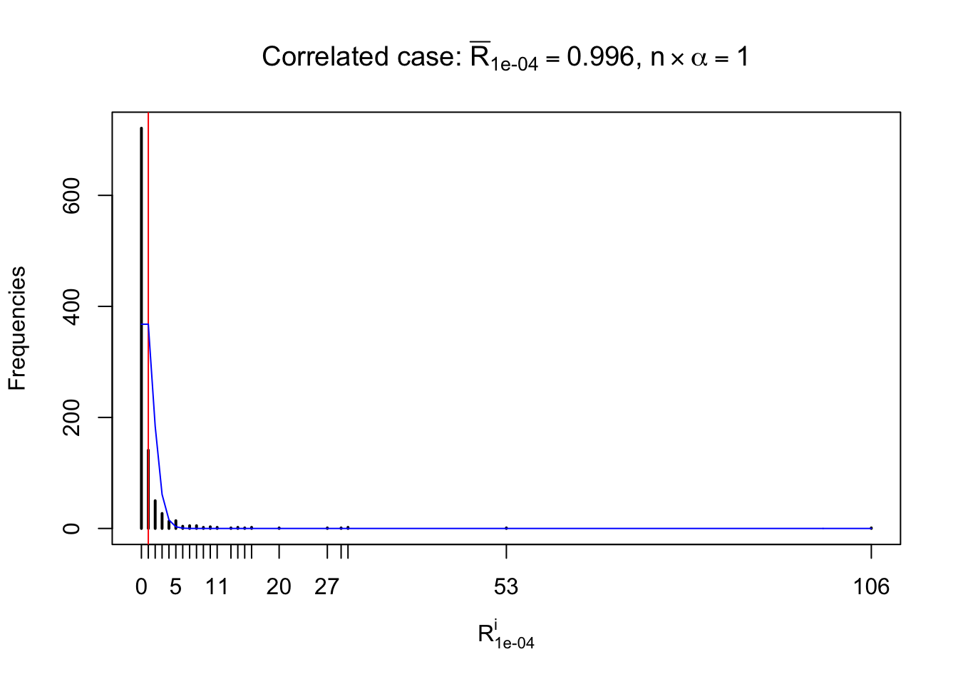
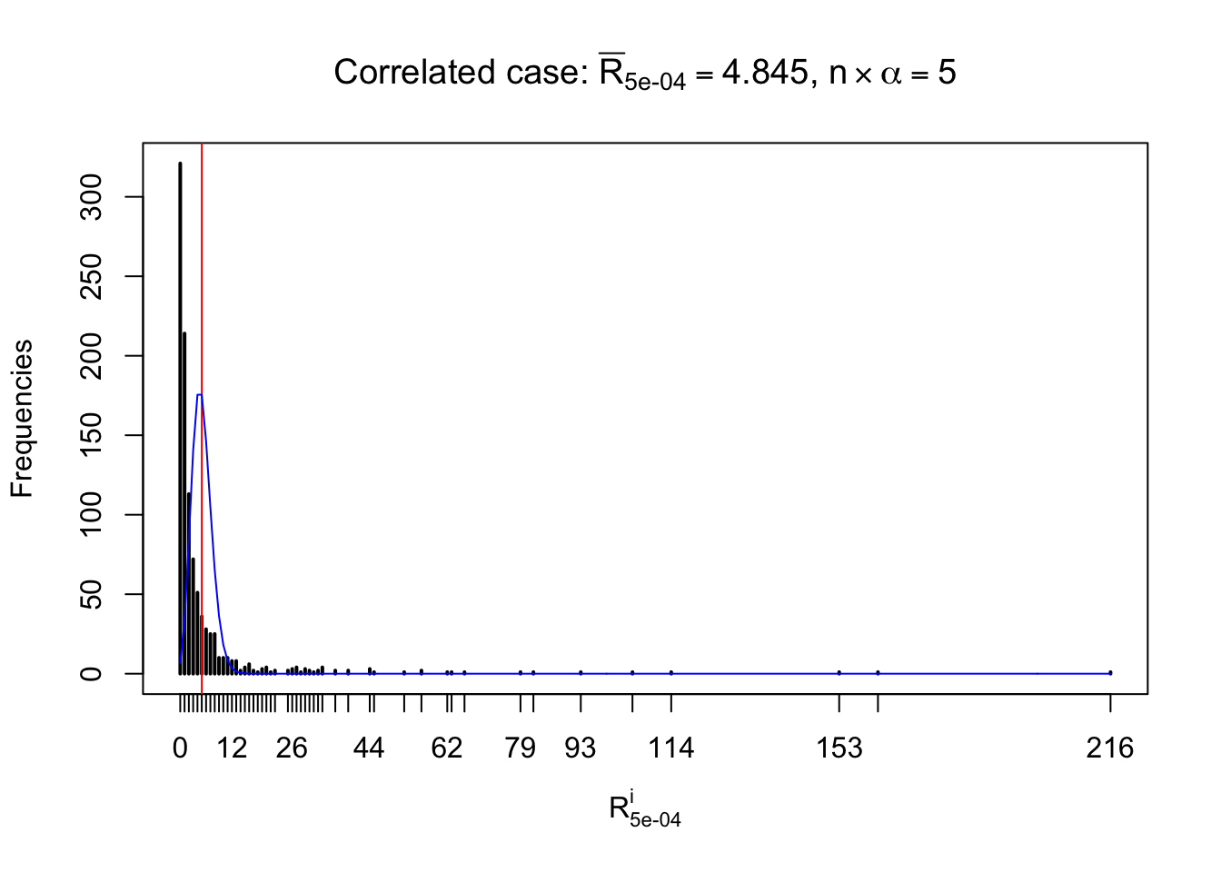
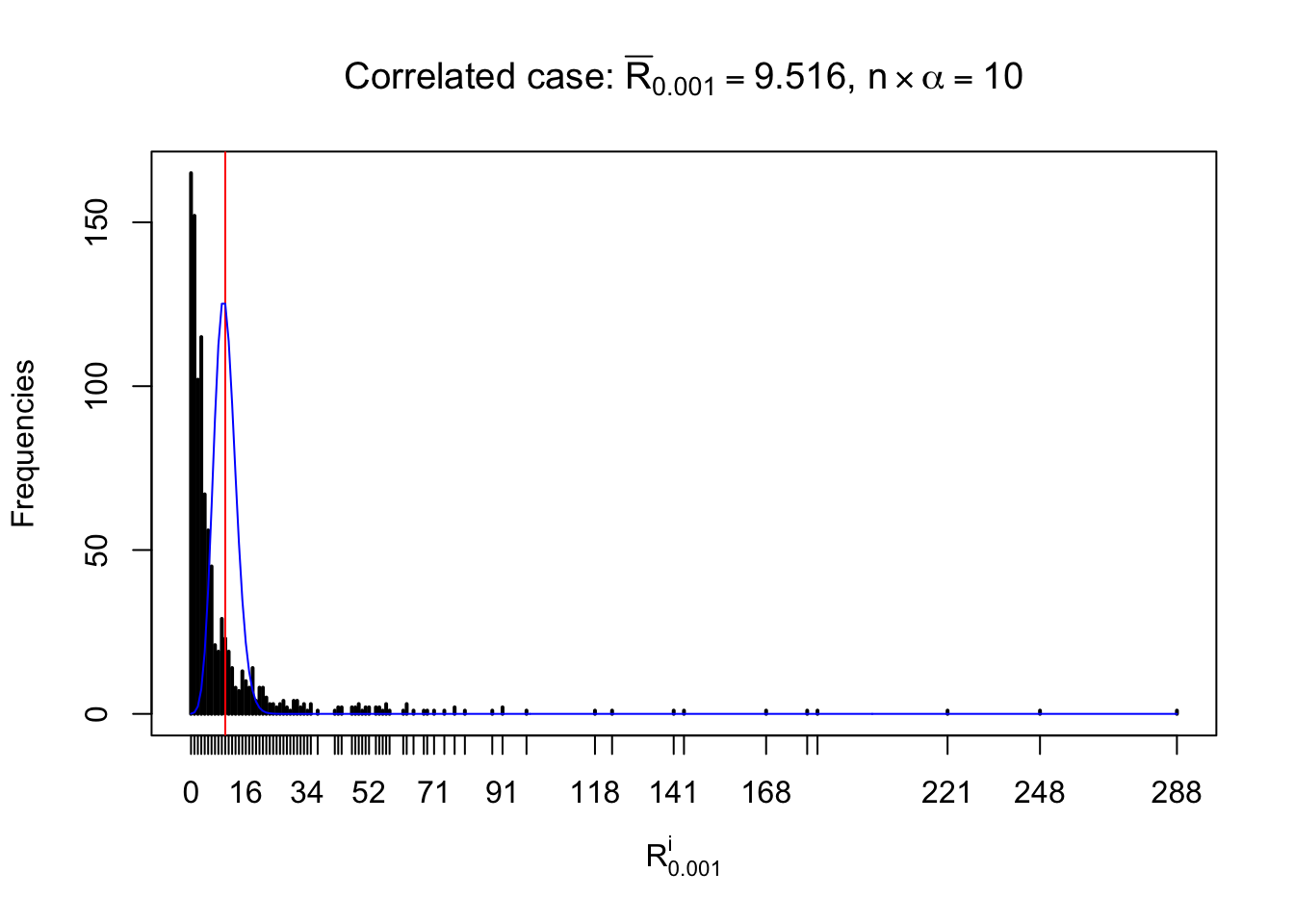
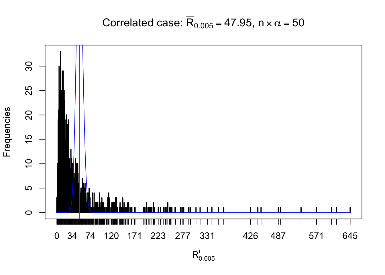
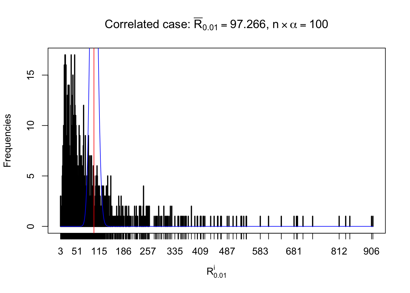
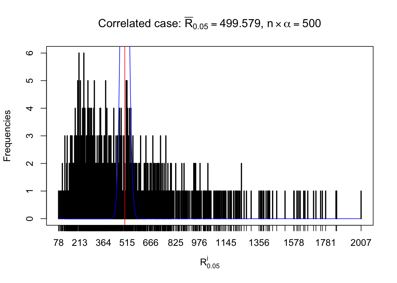
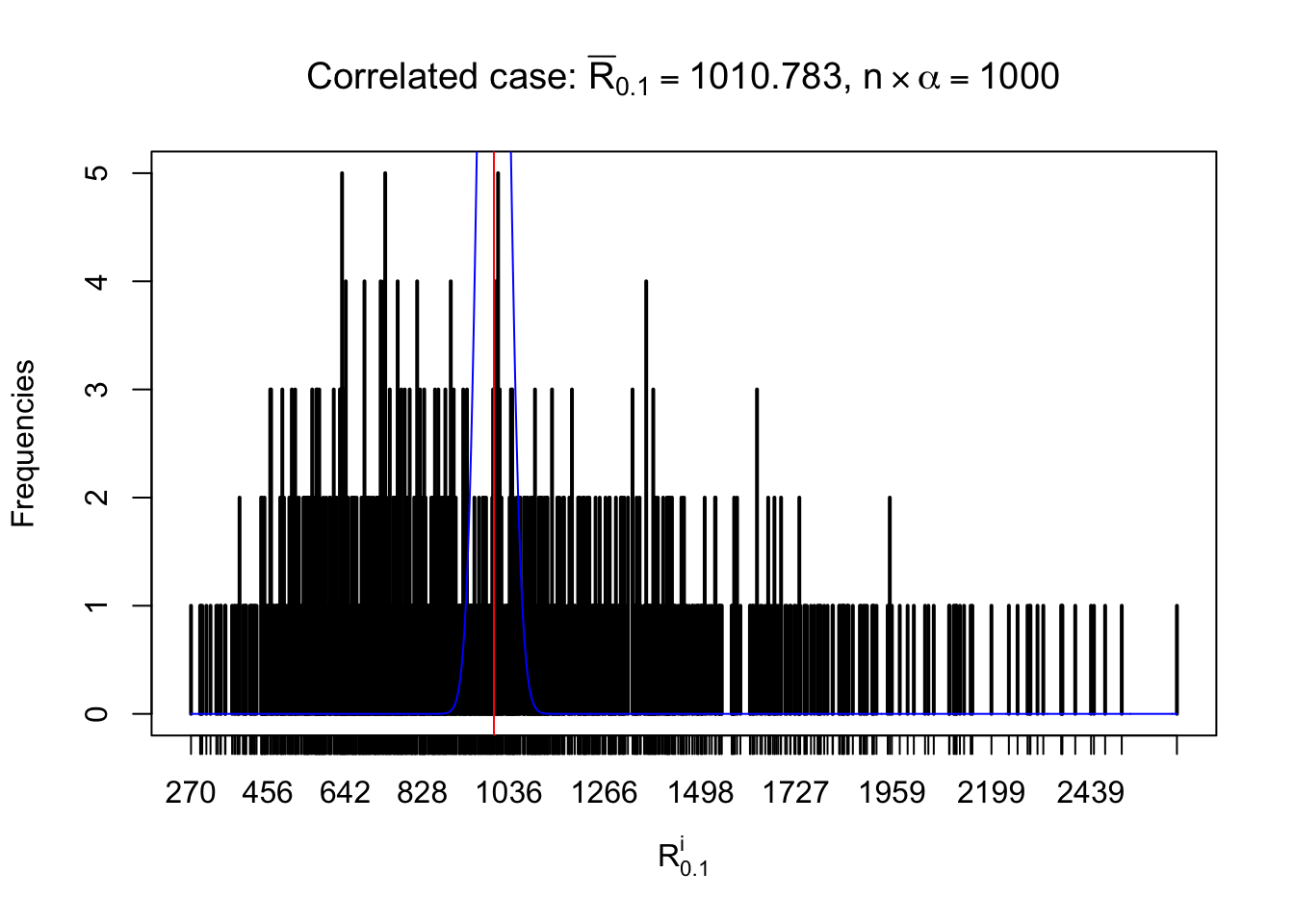
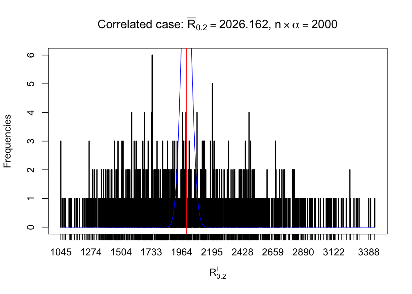
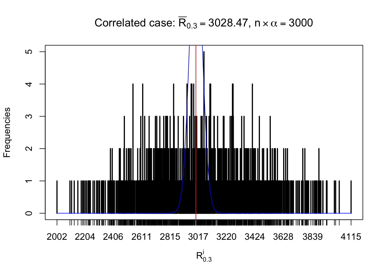
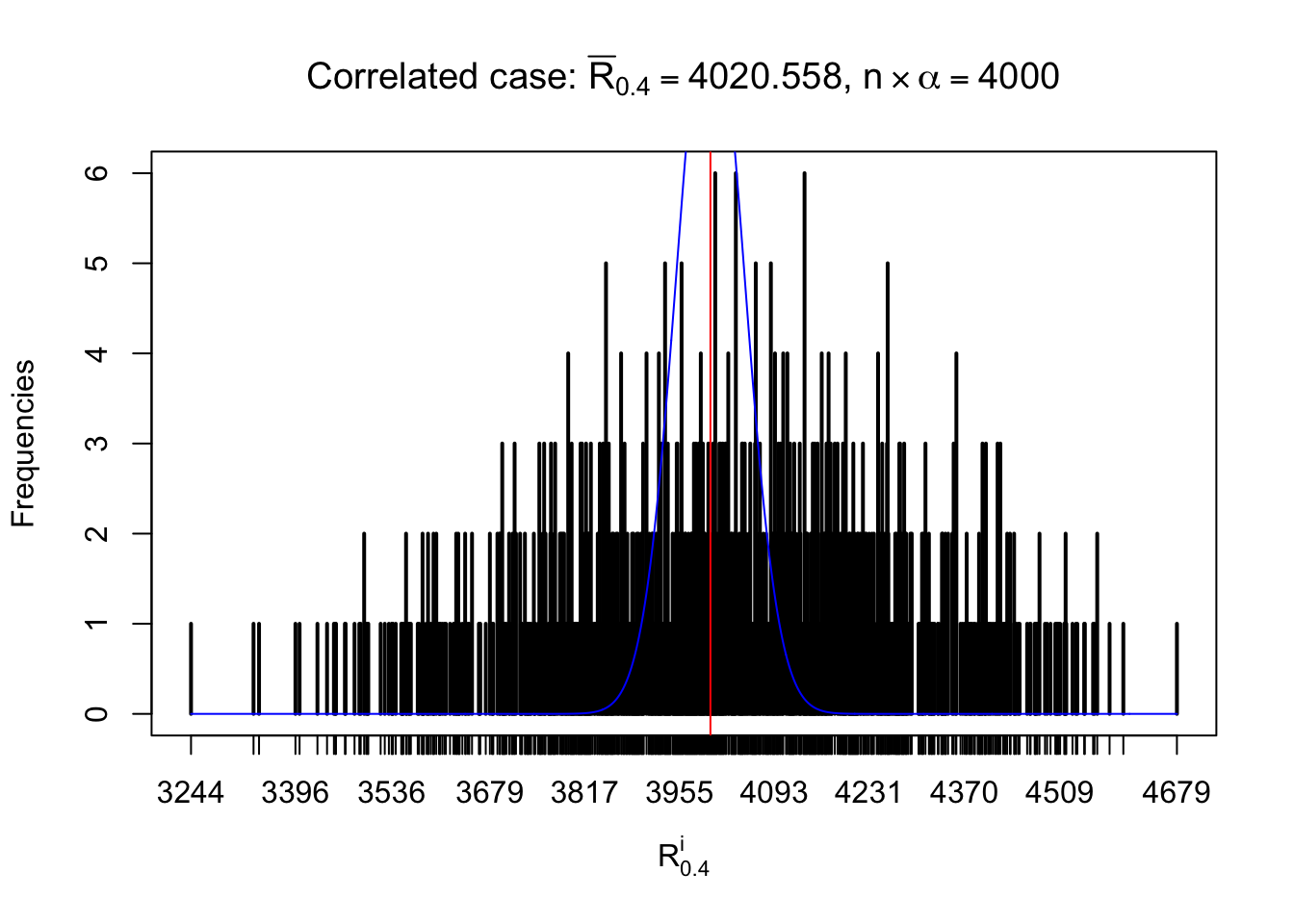
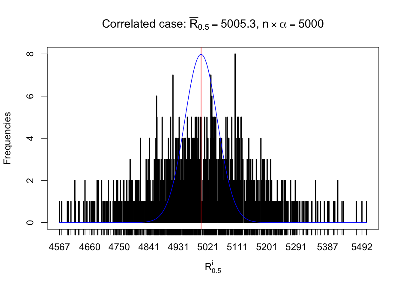
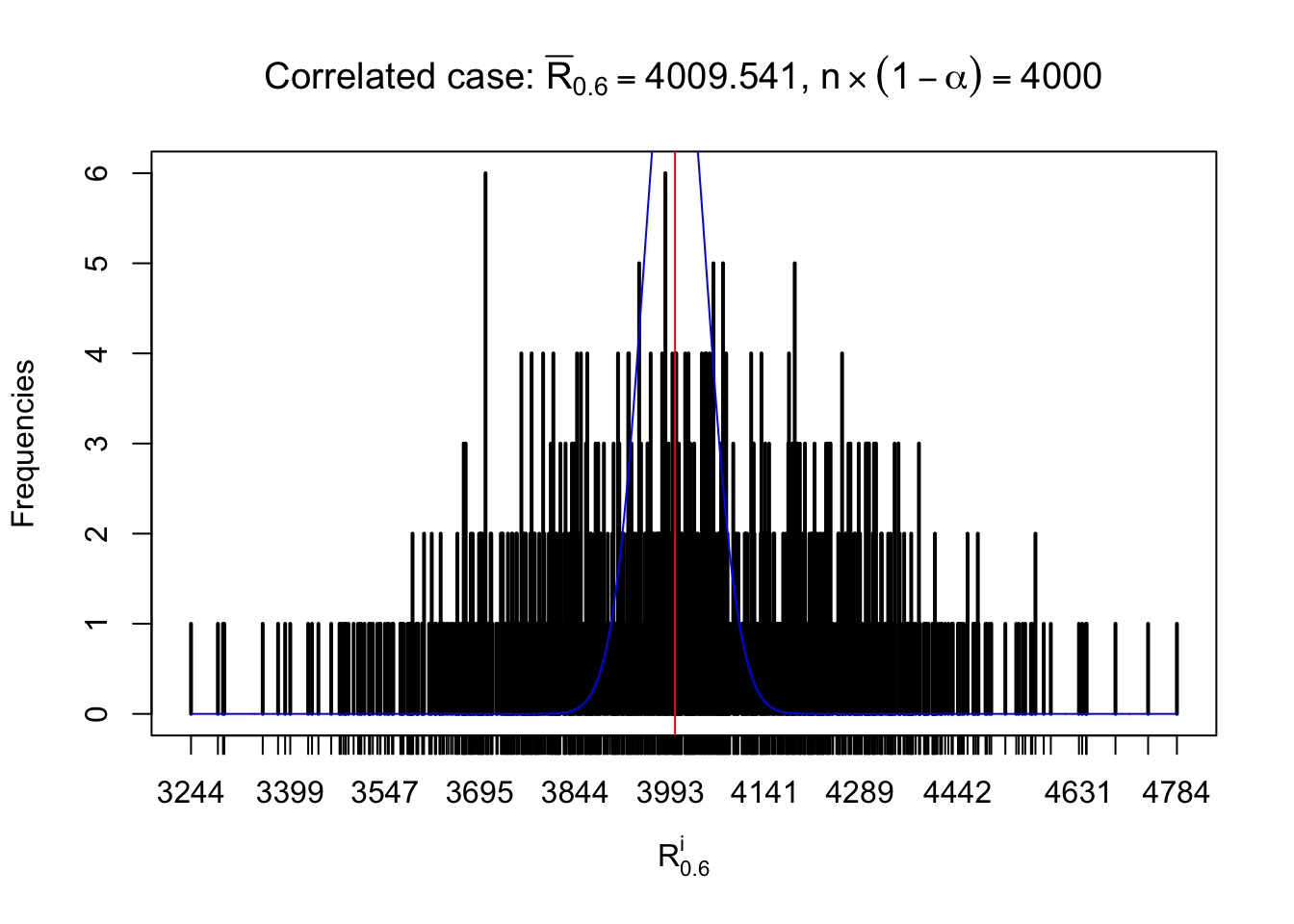
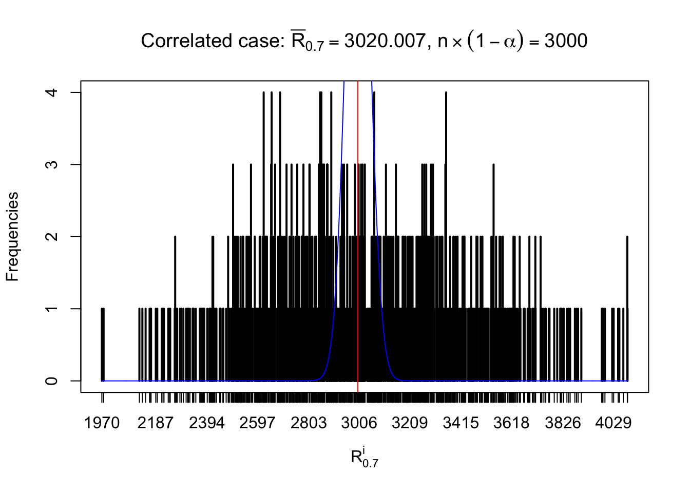
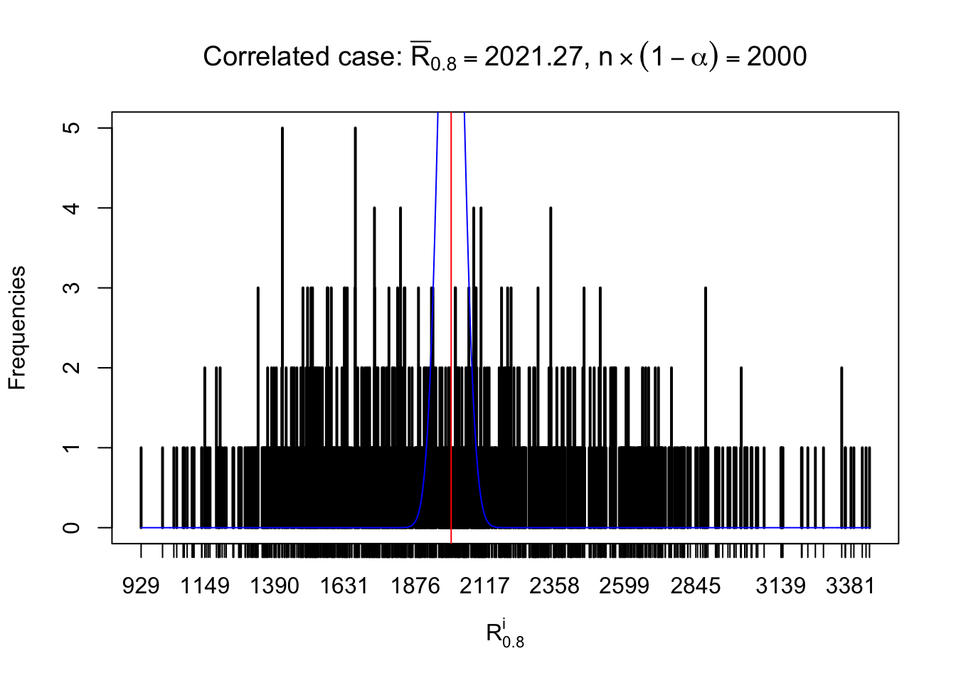
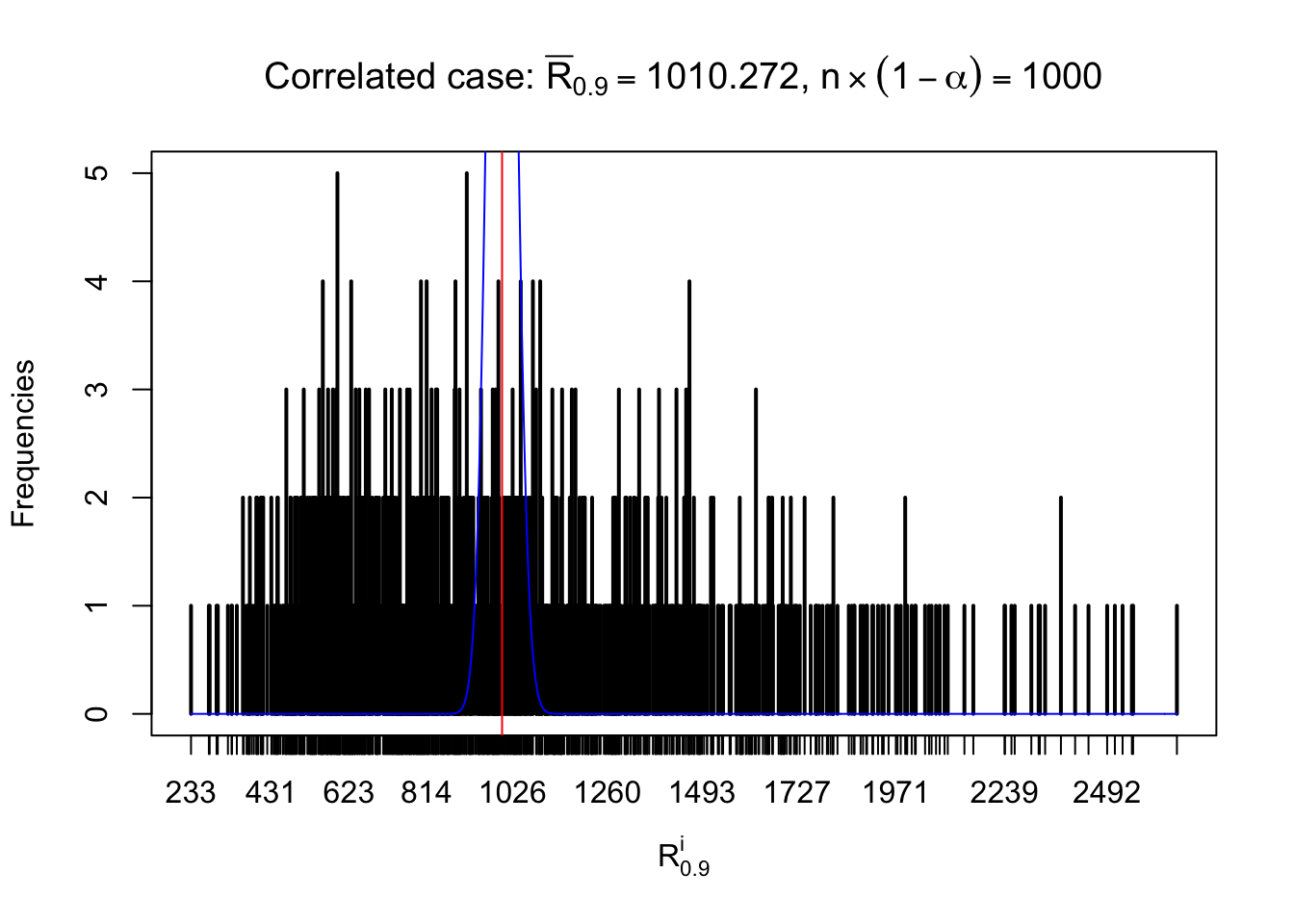
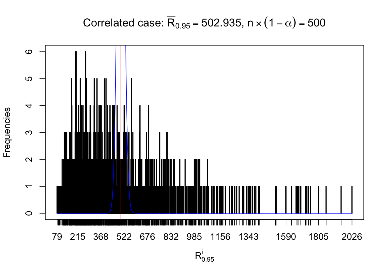
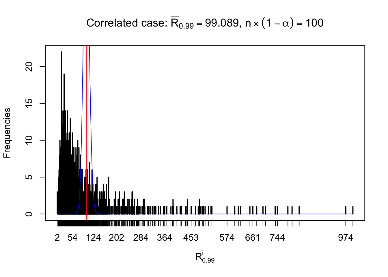
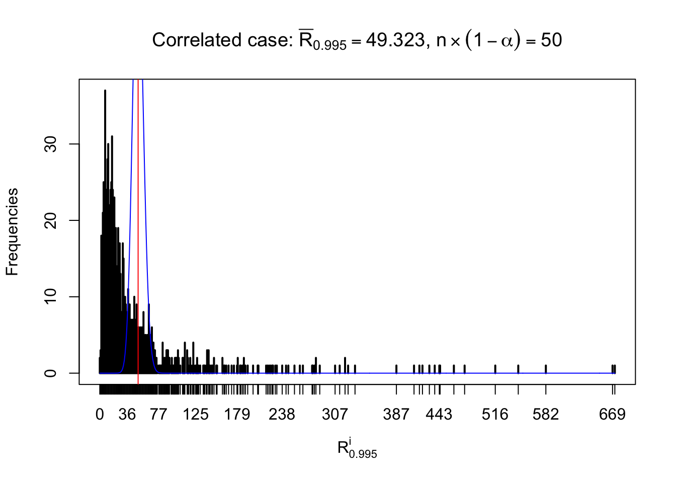
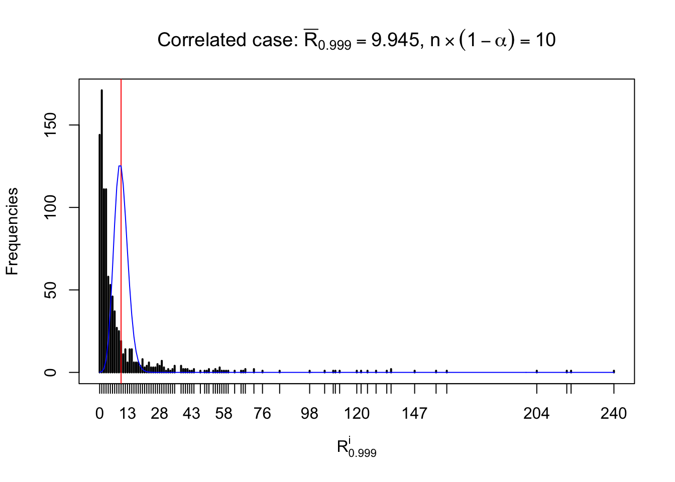
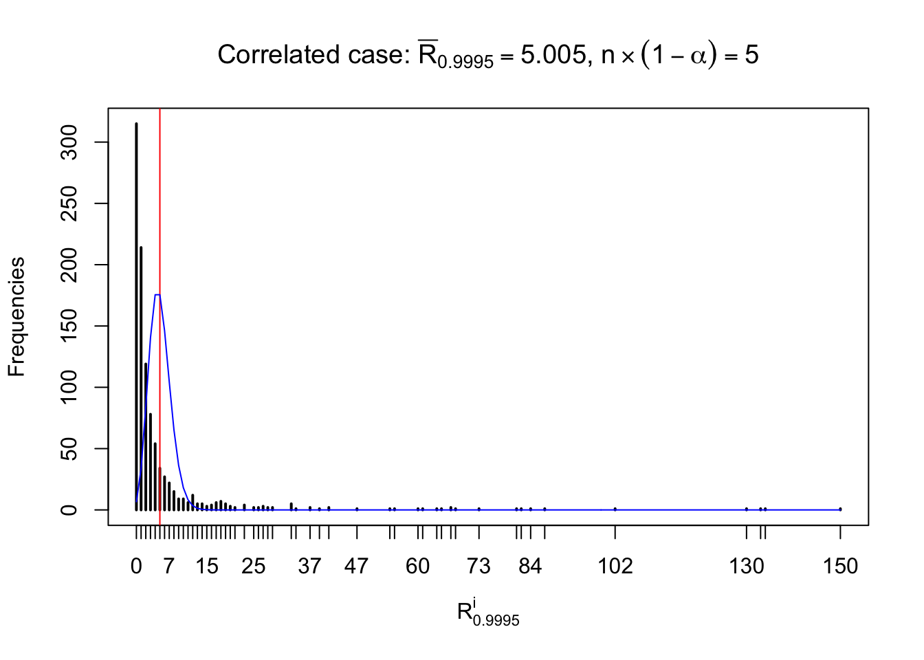
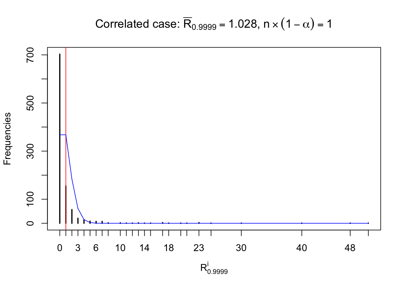
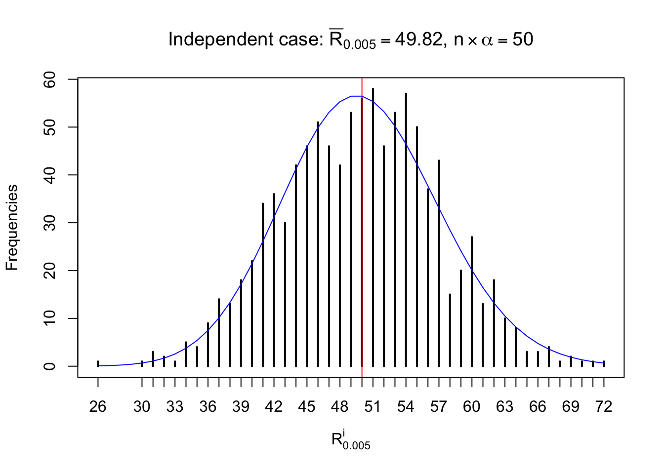
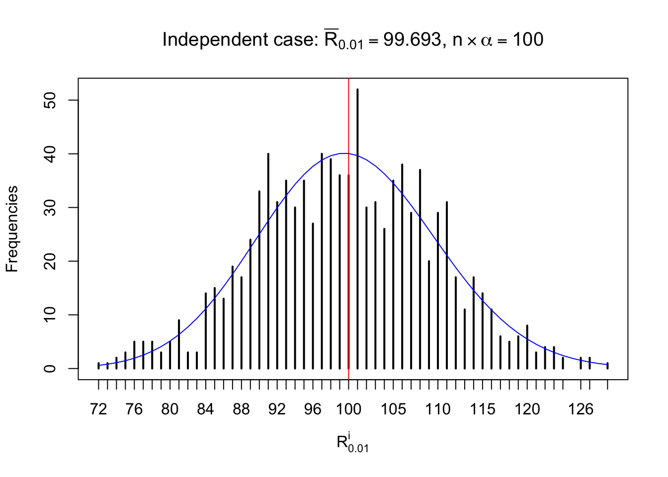
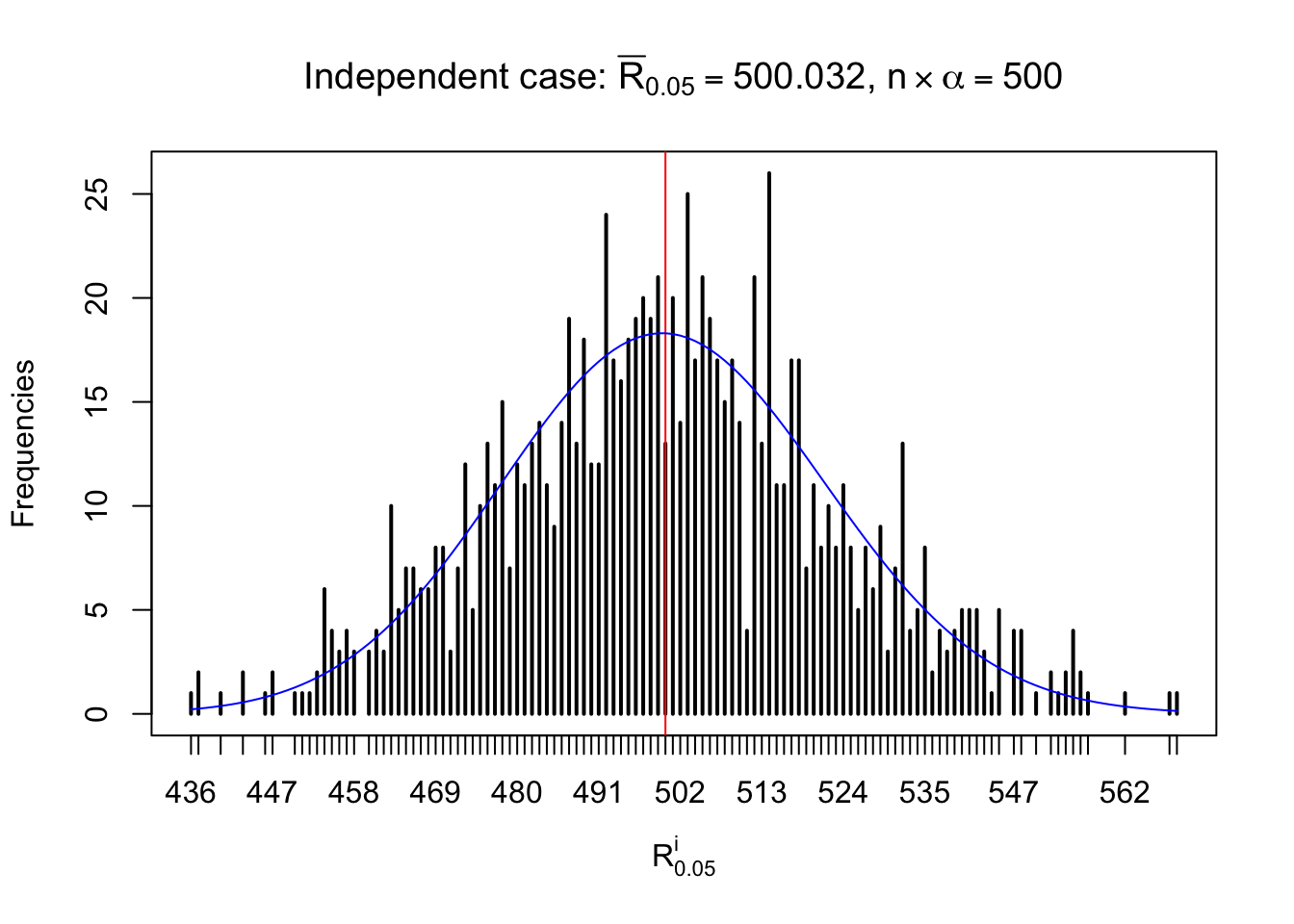
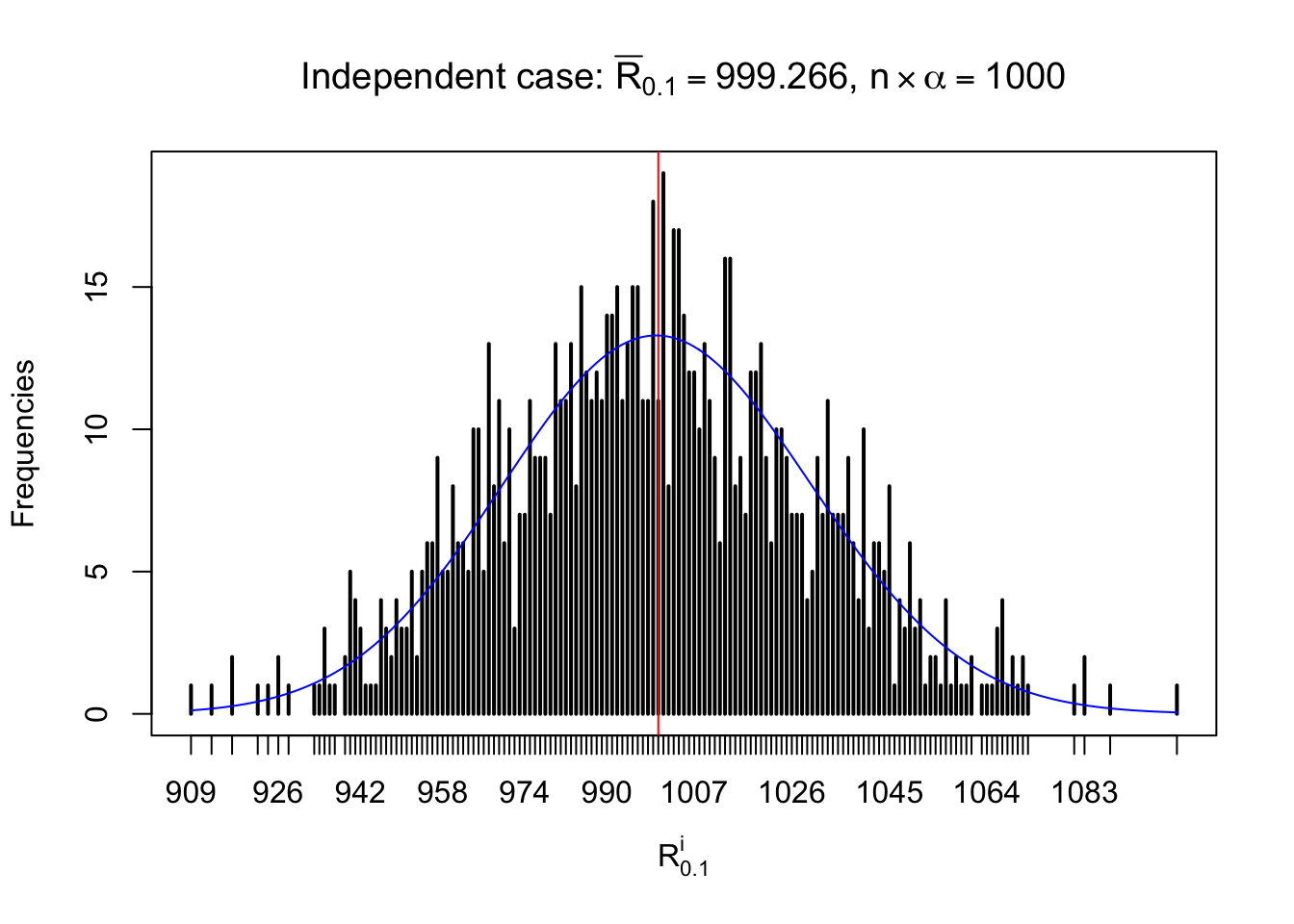
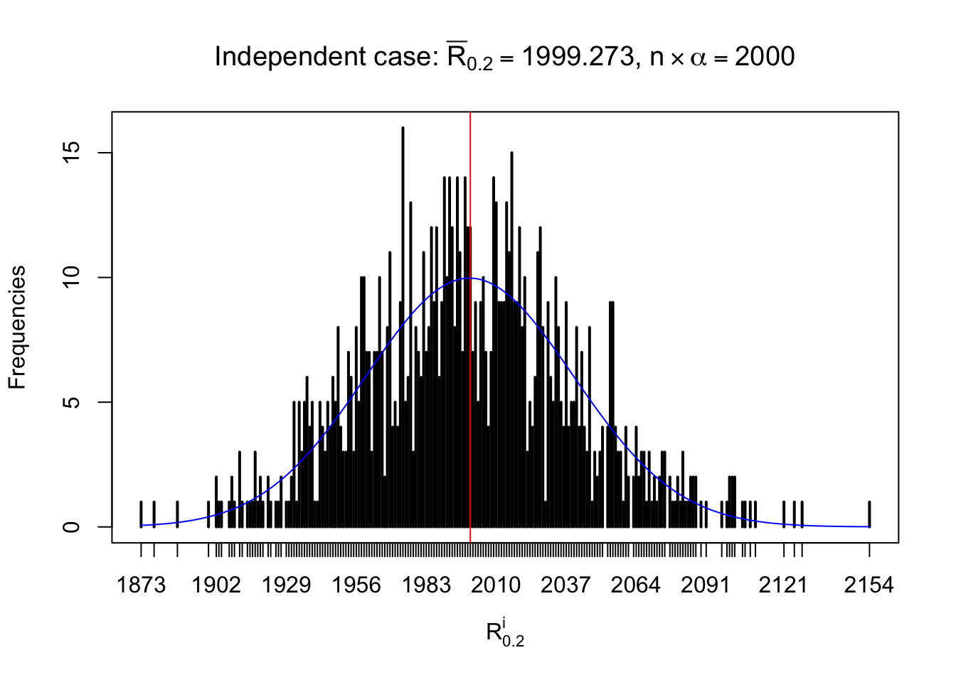
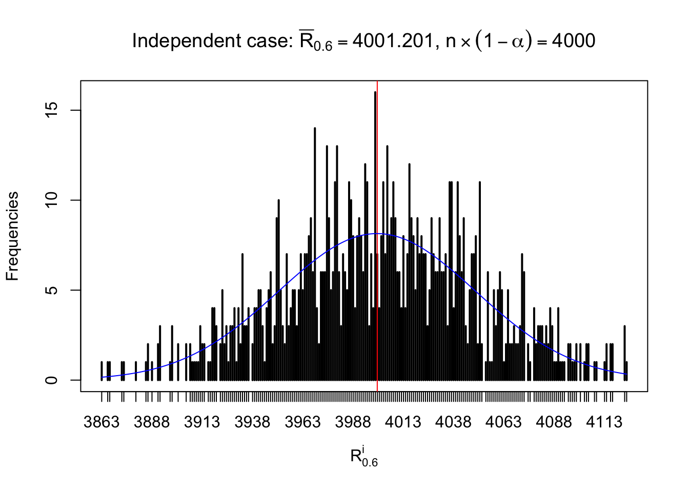
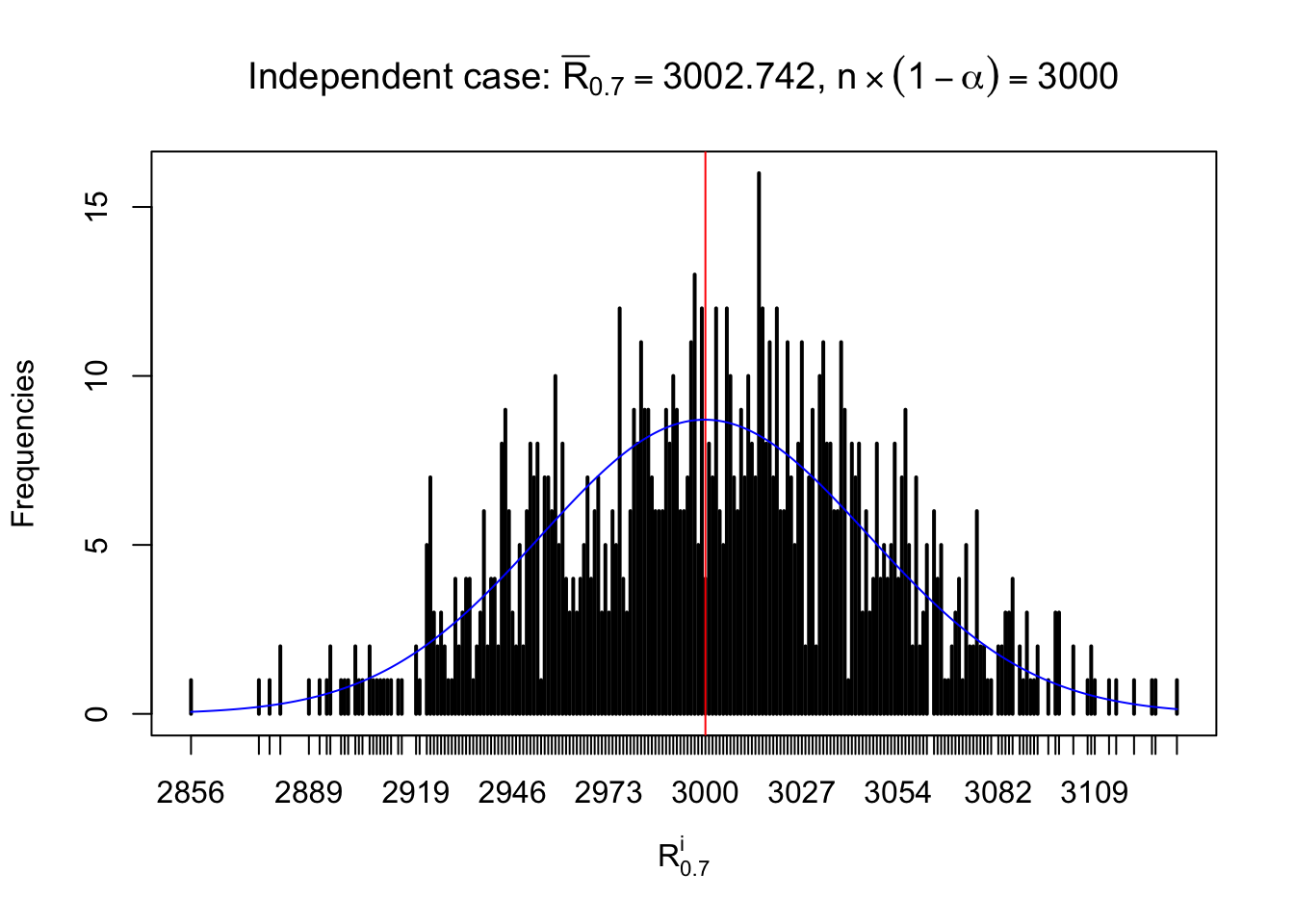
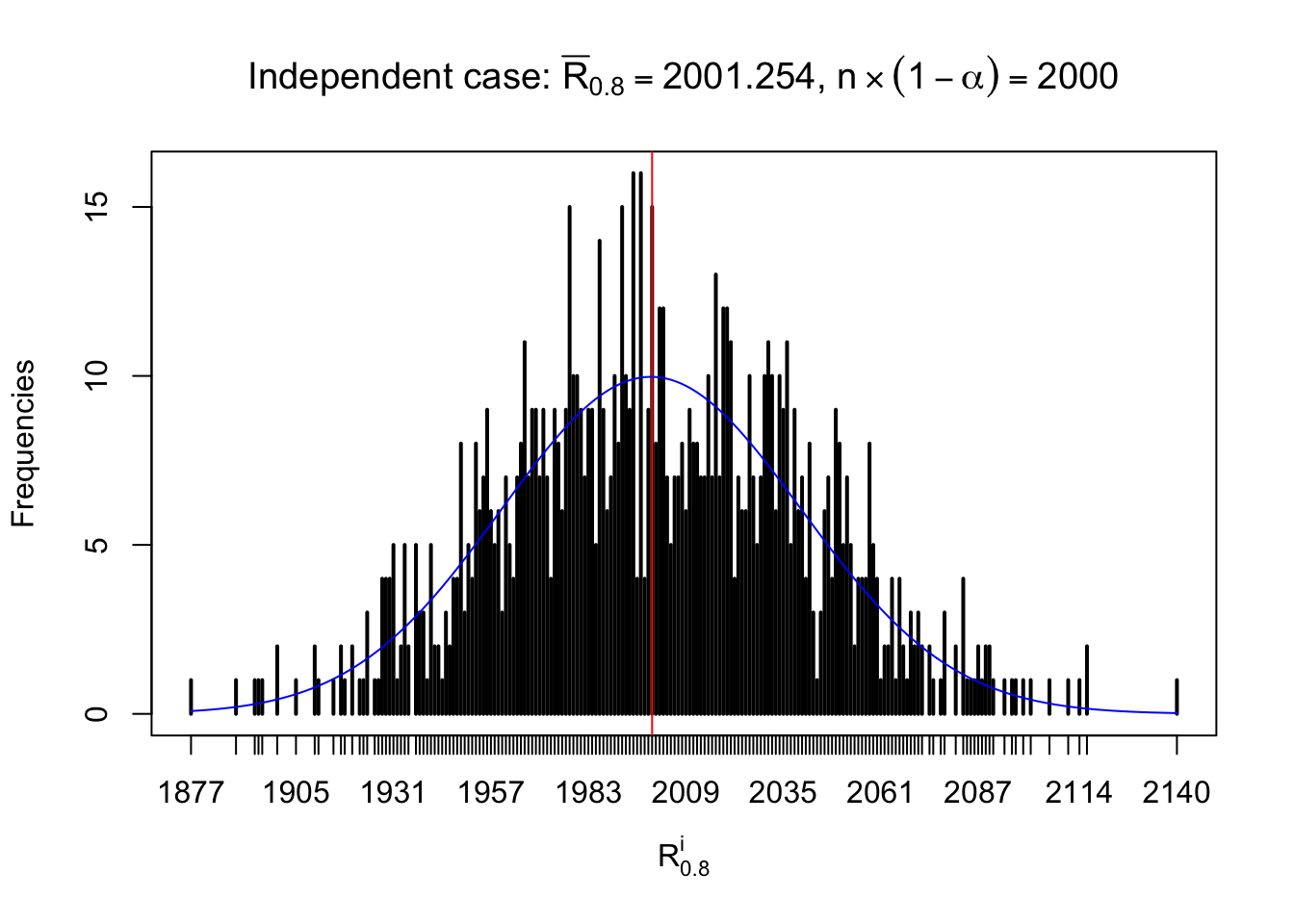
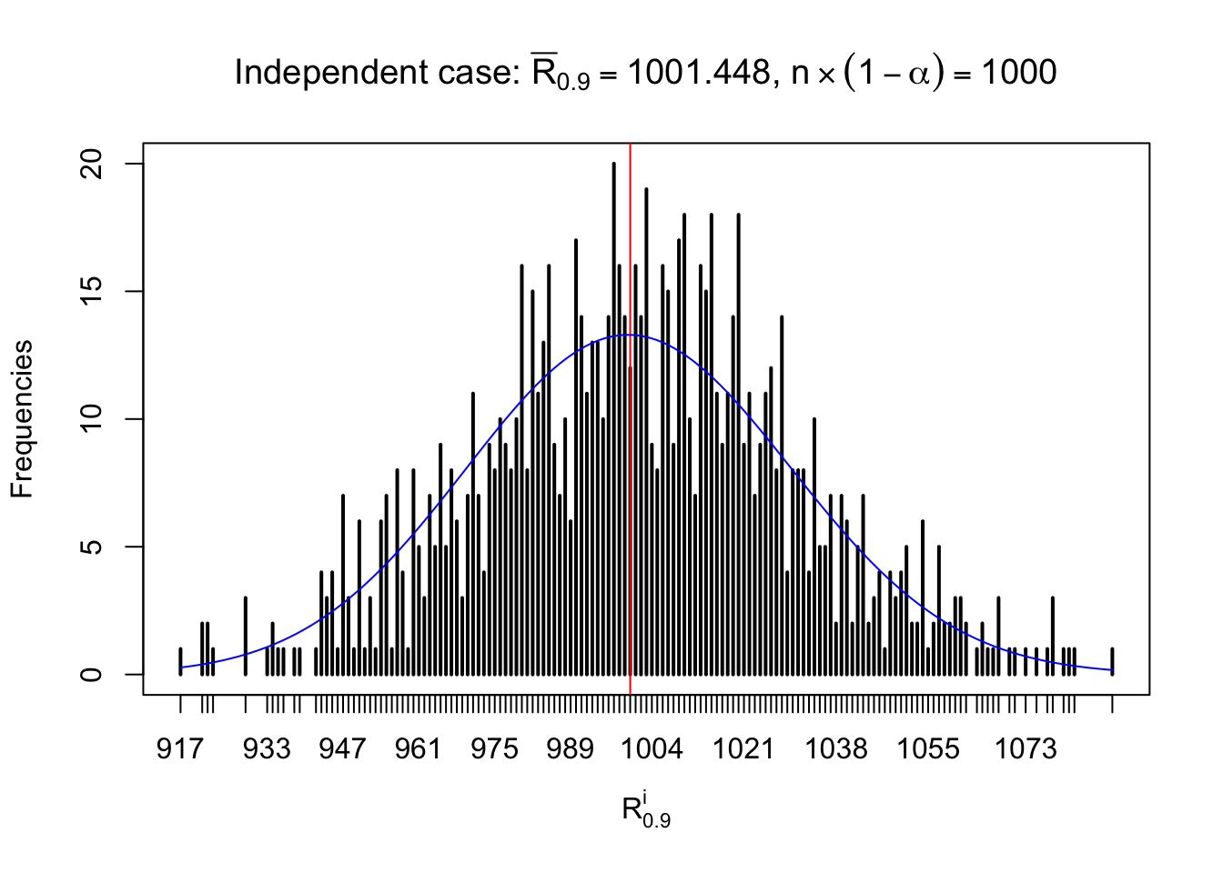
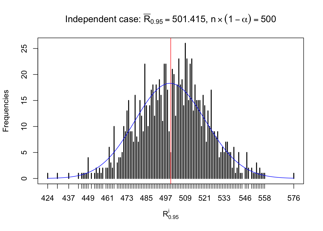
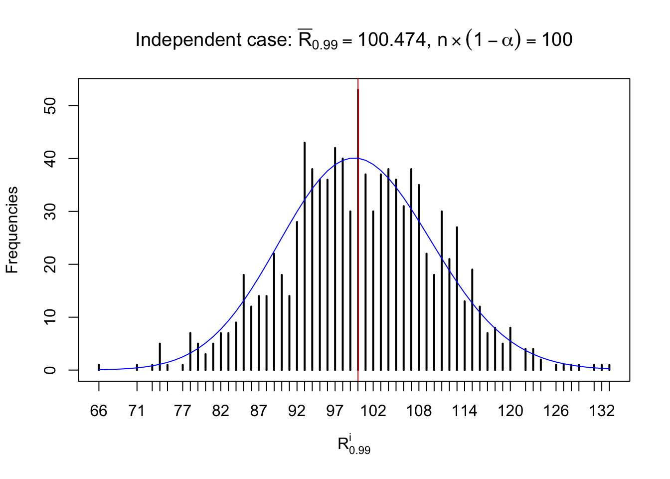
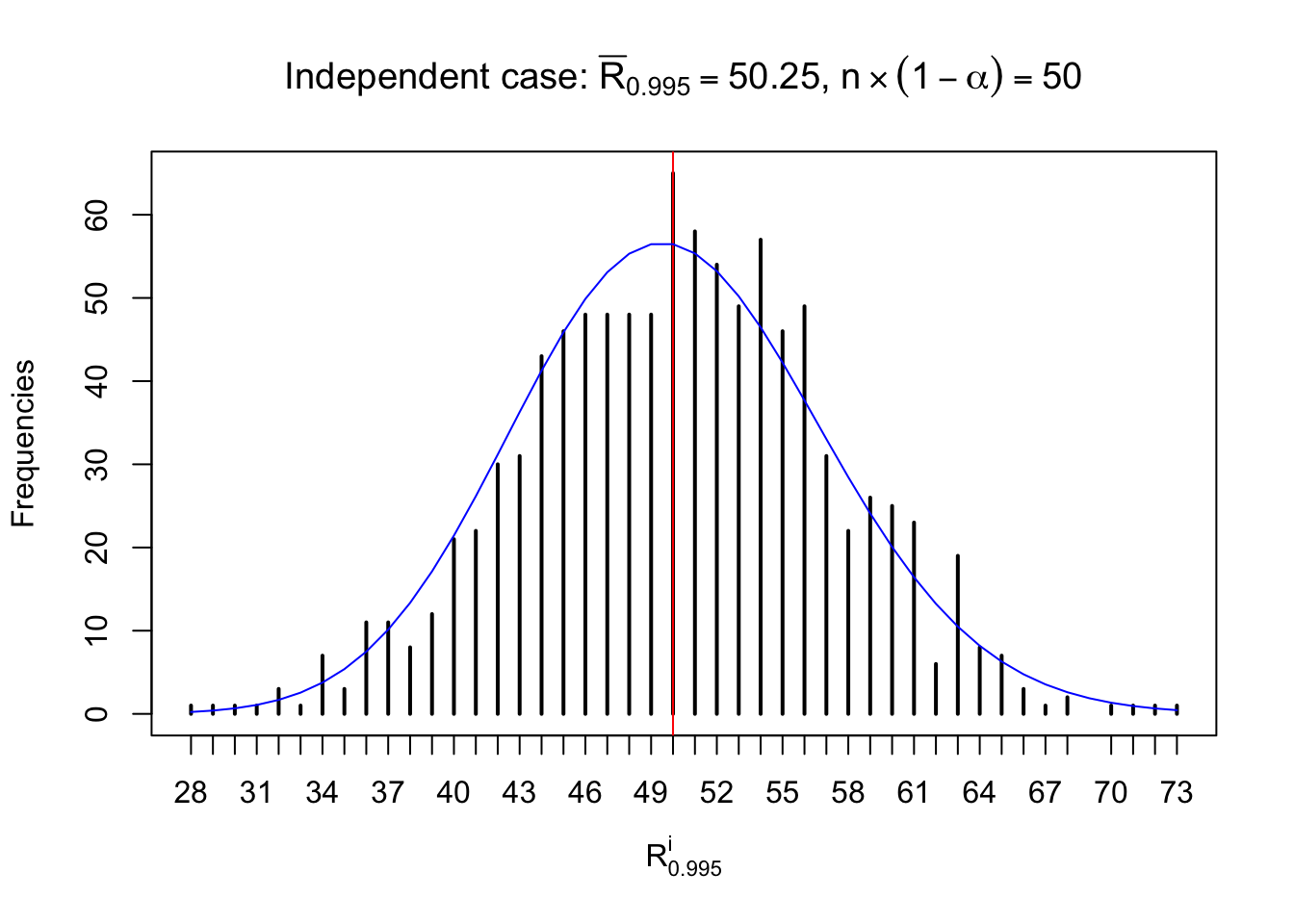
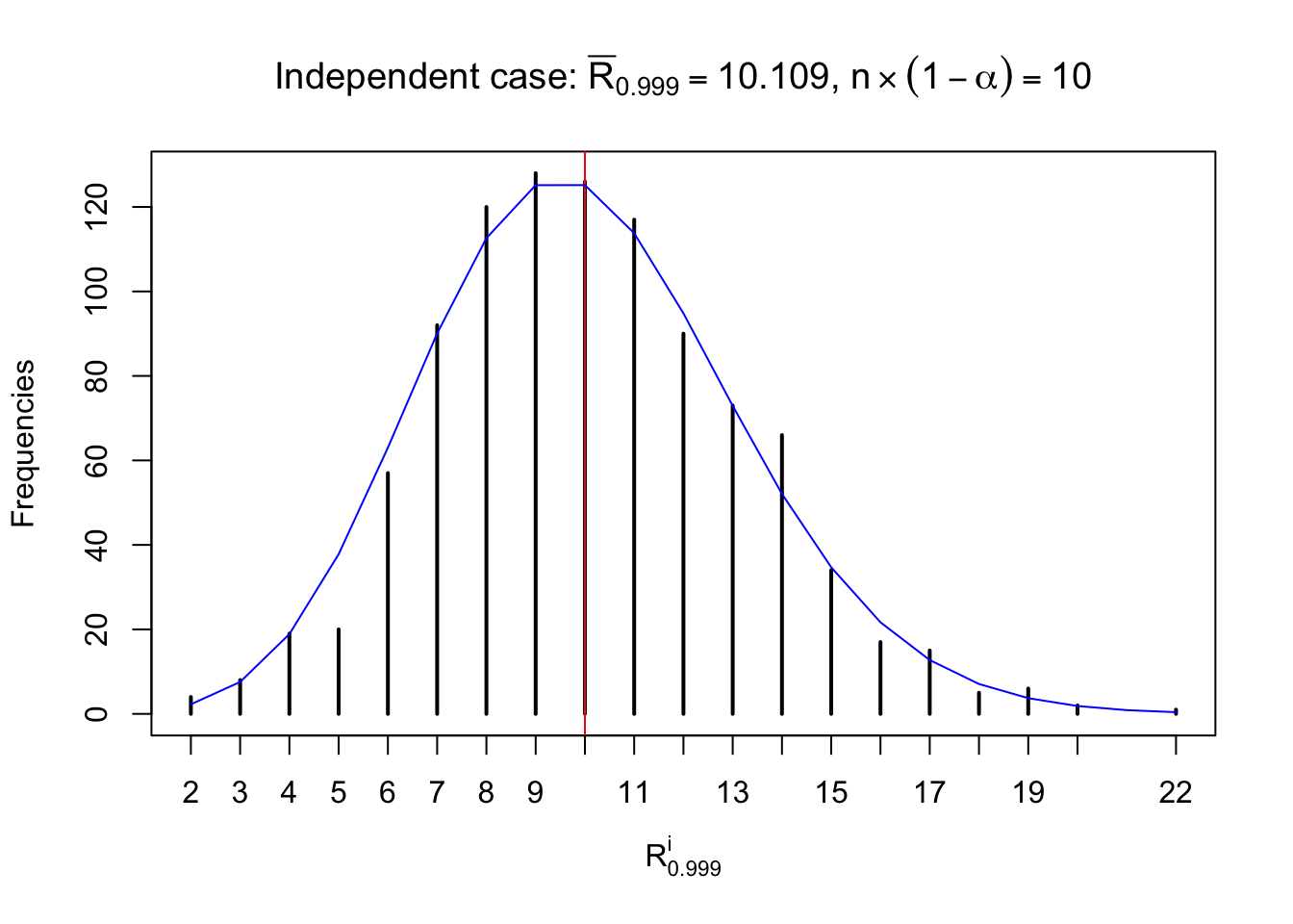
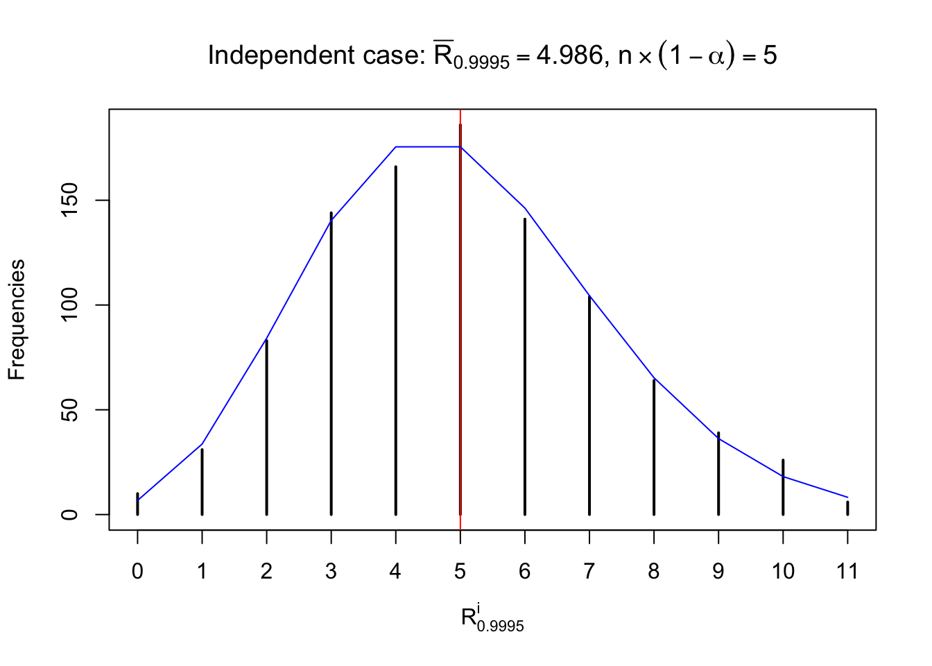
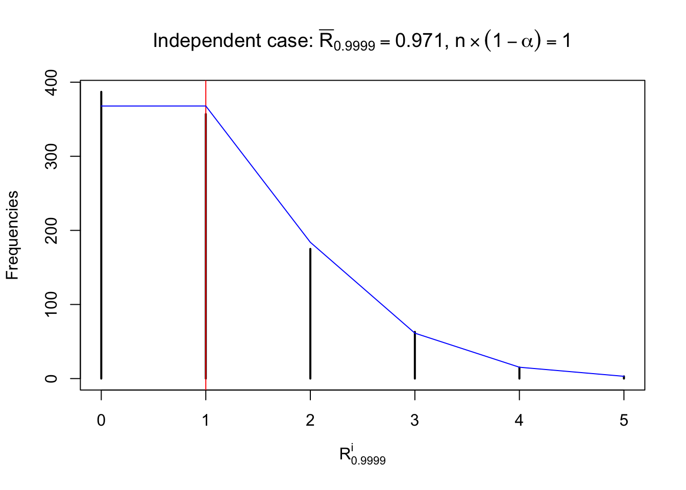
For each row, let \(\alpha\) be a given probability level, \(z_\alpha = \Phi^{-1}\left(\alpha\right)\) be the associated quantile, and we record a number \(R_i^\alpha\) defined as follows.
If \(\alpha \leq 0.5\), \(R_\alpha^i\) is the number of \(z\) scores in row \(i\) that are smaller than \(z_\alpha\); otherwise, if \(\alpha > 0.5\), \(R_\alpha^i\) is the number of \(z\) scores in row \(i\) that are larger than \(z_\alpha\).
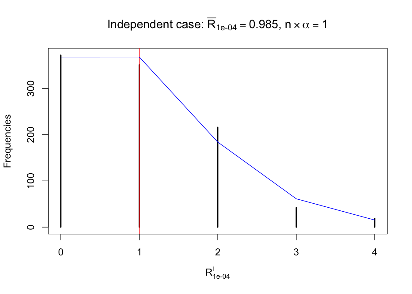
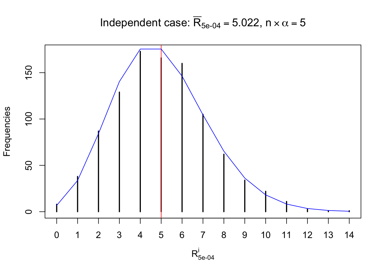
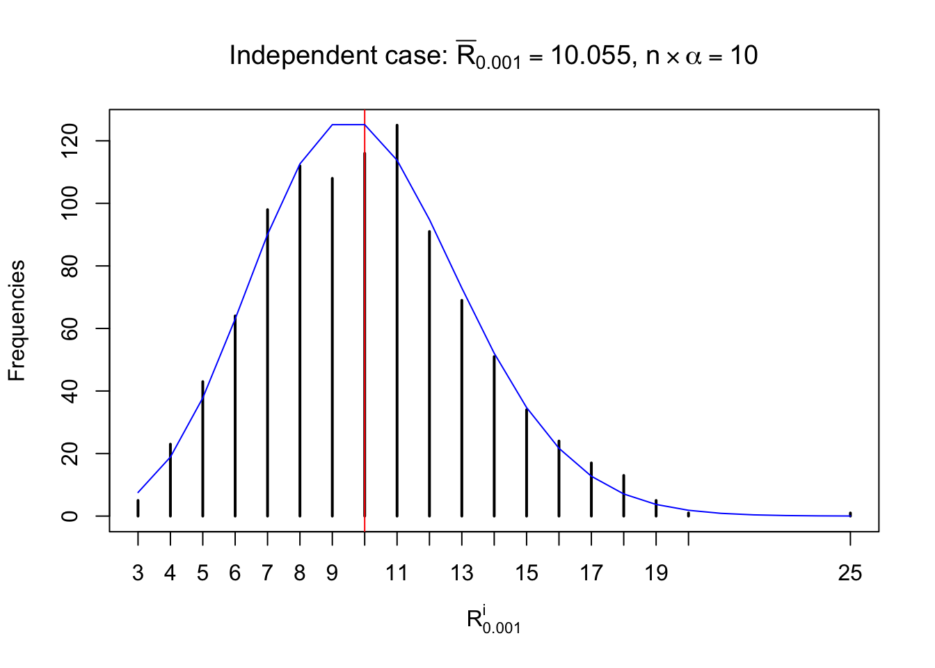
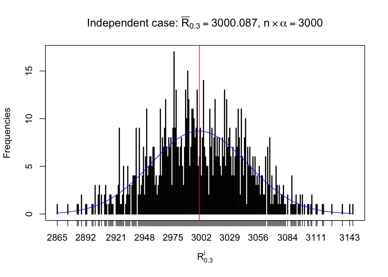
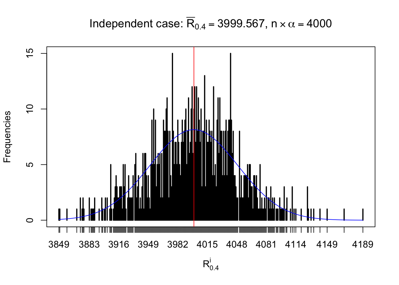
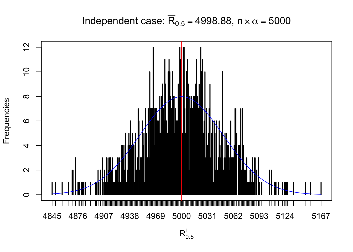
Defined this way, \(R_\alpha^i\) should be a sample from \(n \times F_n^{R_i}\left(z_\alpha\right)\) or \(n \times \left(1- F_n^{R_i}\left(z_\alpha\right)\right)\). We can check if \(E\left[F_n\left(z\right)\right] = \Phi\left(z\right)\) by looking at if the average \[ \bar R_\alpha \approx \begin{cases} n\Phi\left(z_\alpha\right) = n\alpha & \alpha \leq 0.5 \\ n\left(1-\Phi\left(z_\alpha\right)\right) = n\left(1 - \alpha\right) & \alpha > 0.5\end{cases} \ . \] We may also compare the frequencies of \(R_\alpha^i\) with their theoretical expected values \(m \times \text{Binomial}\left(n, \alpha\right)\) (in blue) assuming \(z_{ij}\) are independent.
Independent case: row-wise
Column-wise: closer to \(N\left(0, 1\right)\)
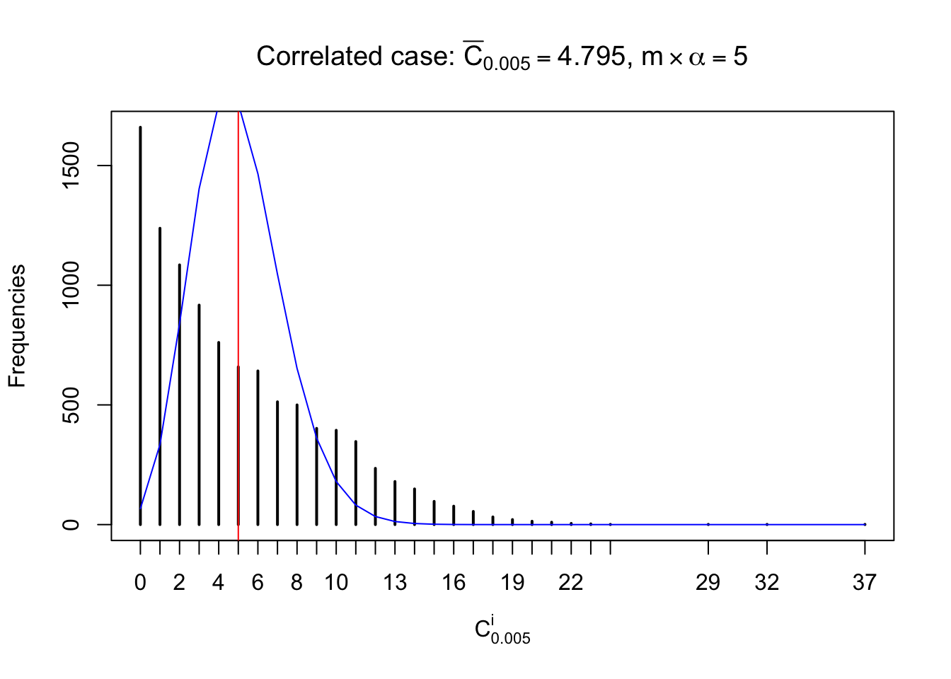
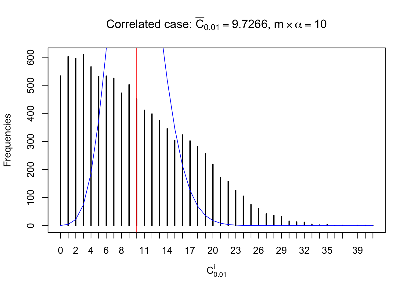
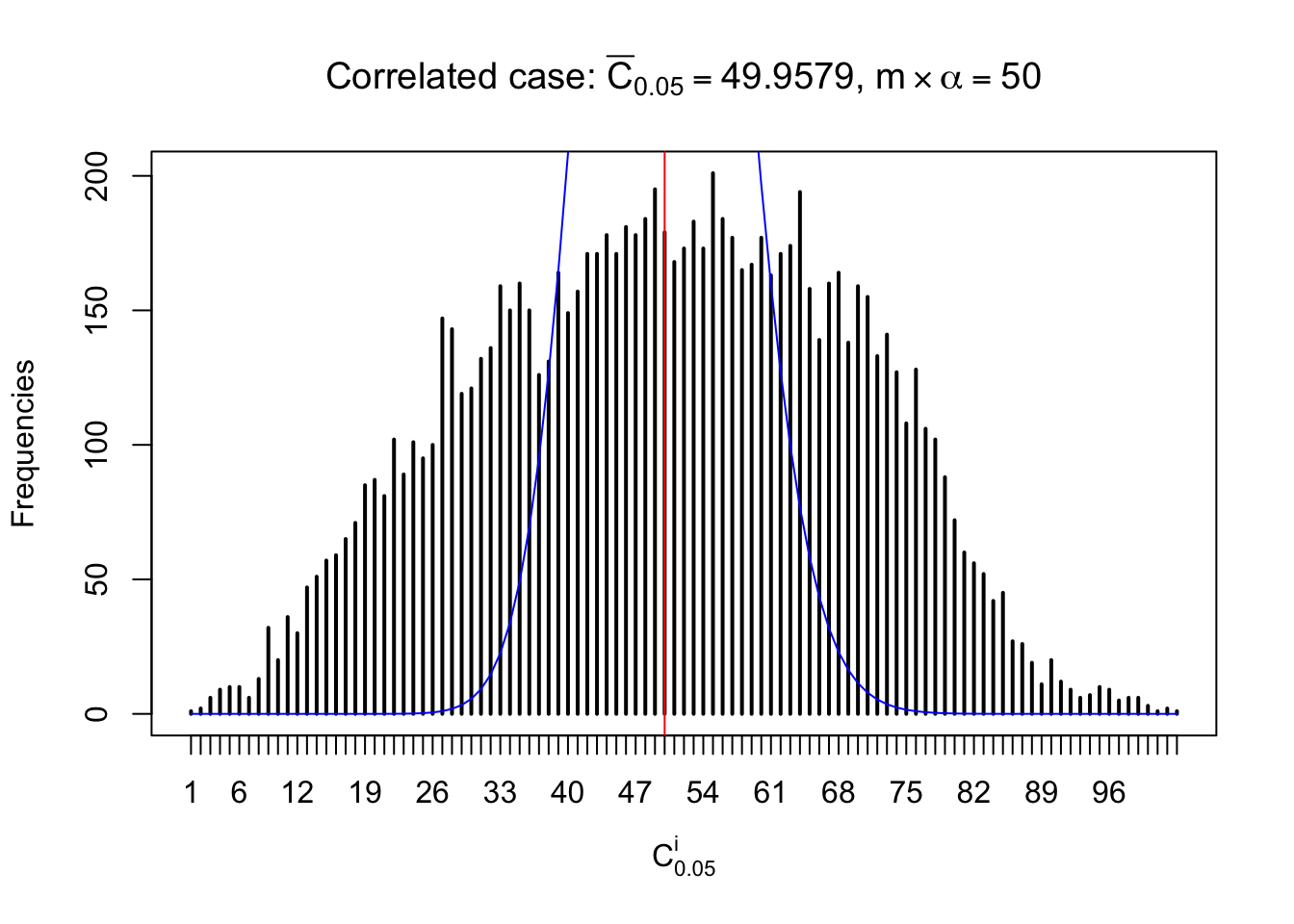
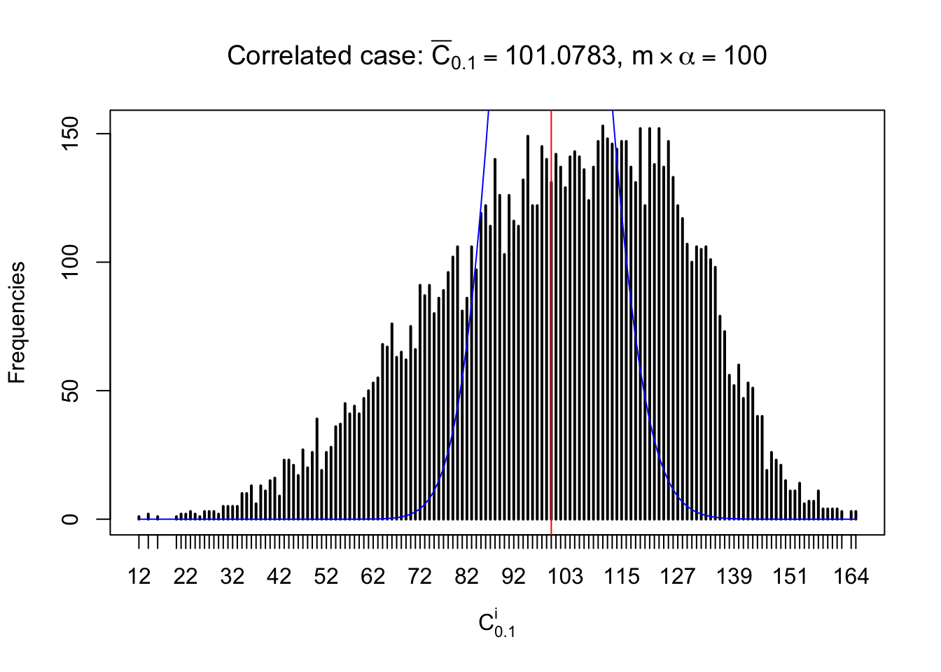
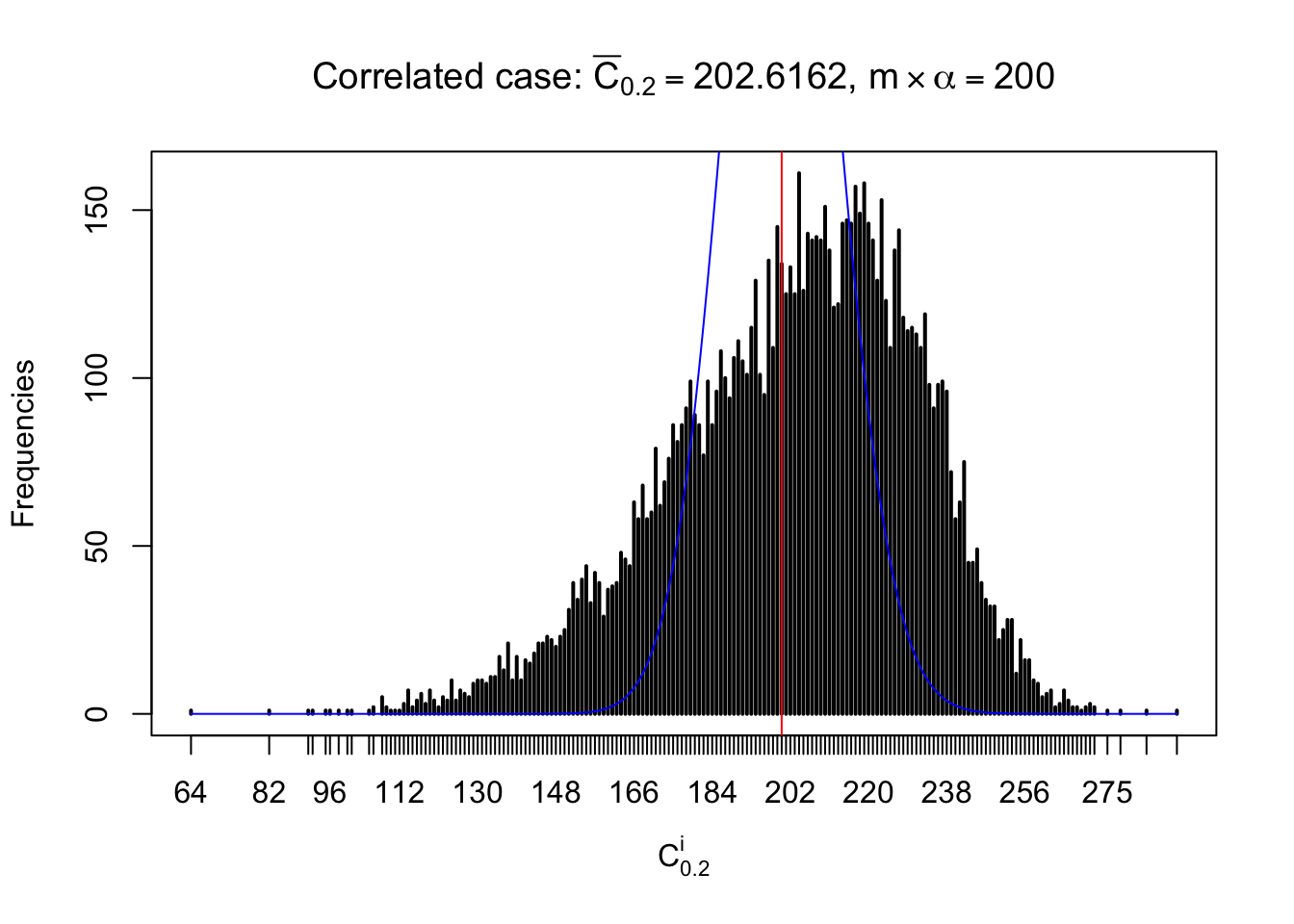
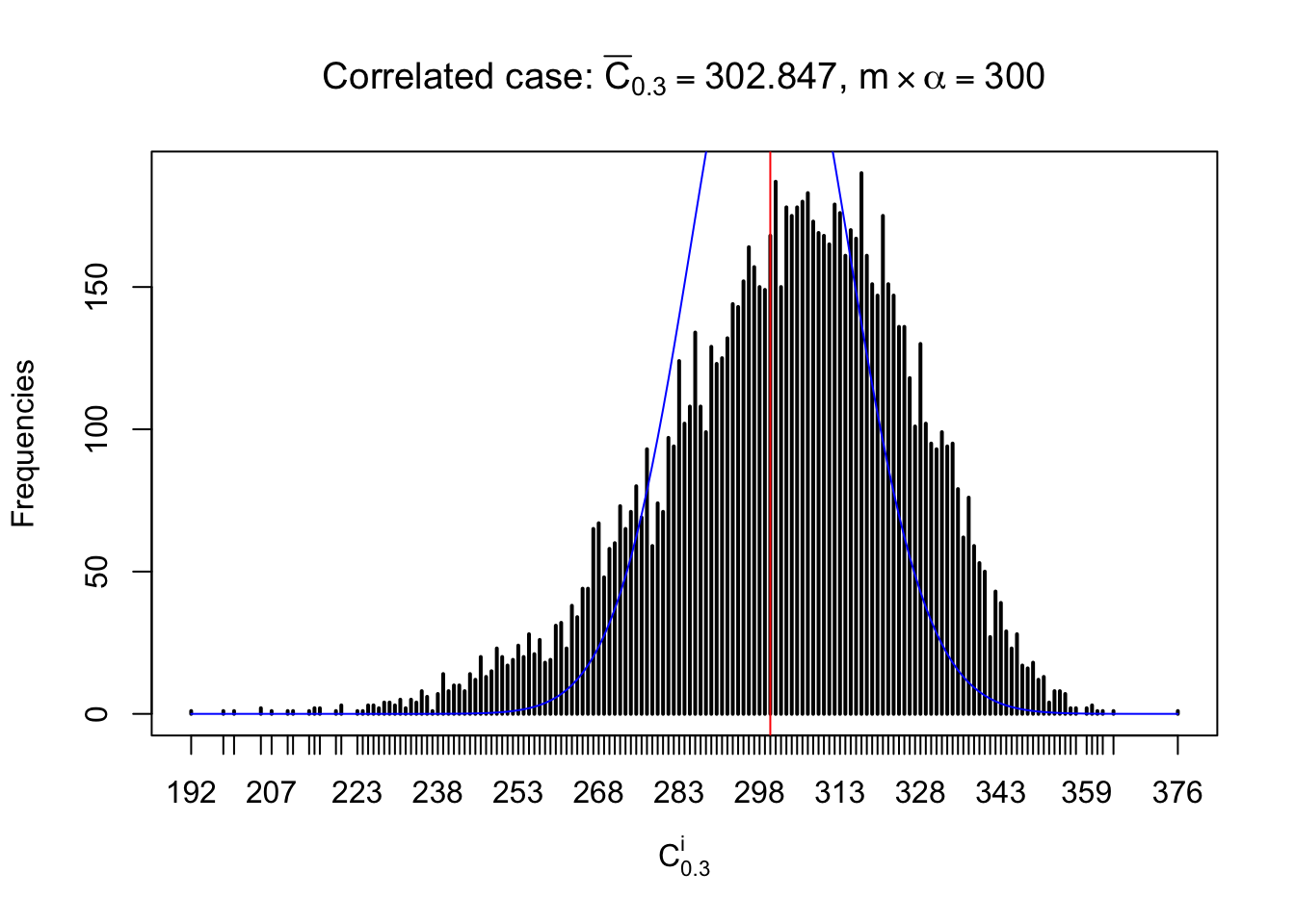
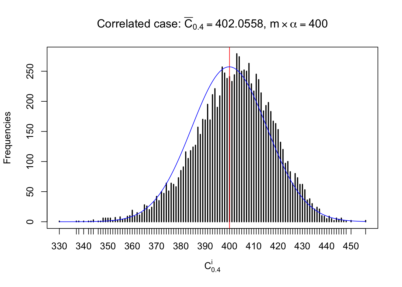
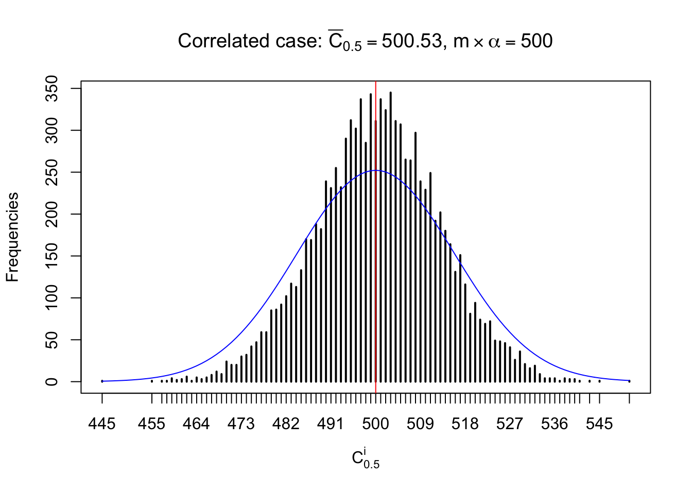
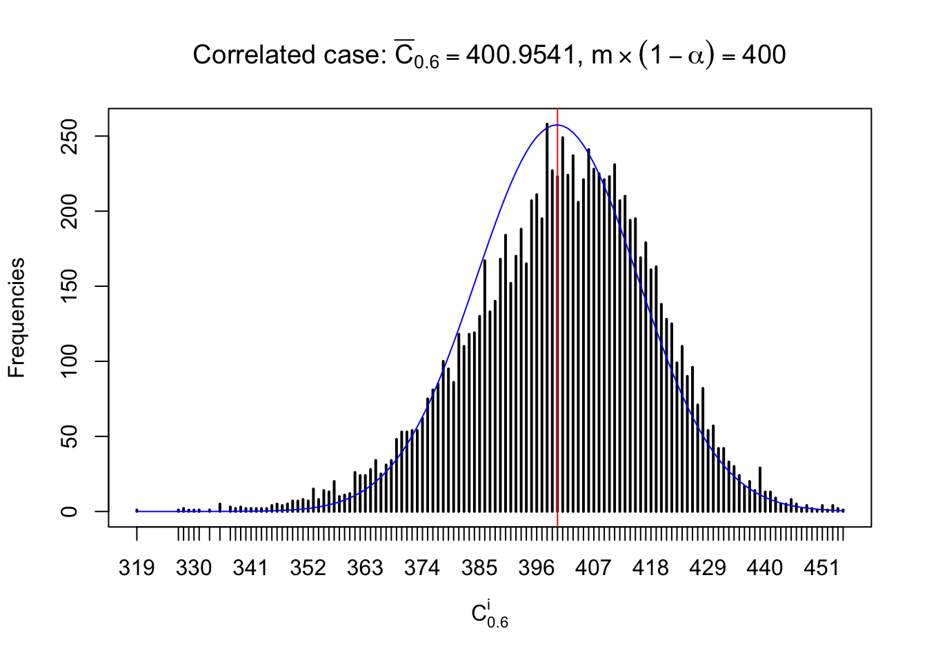
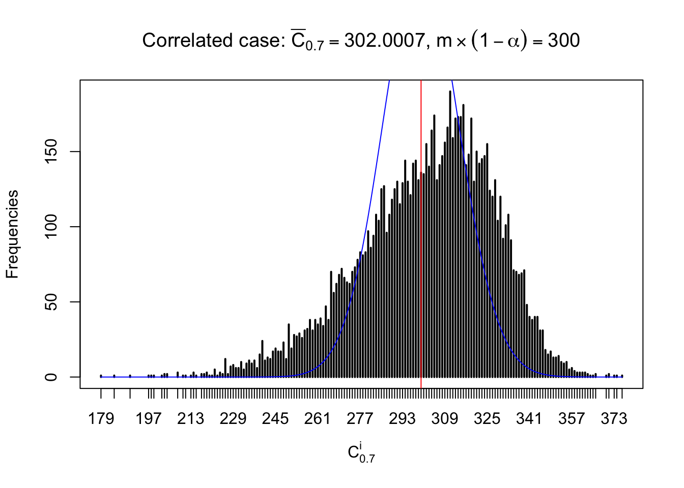
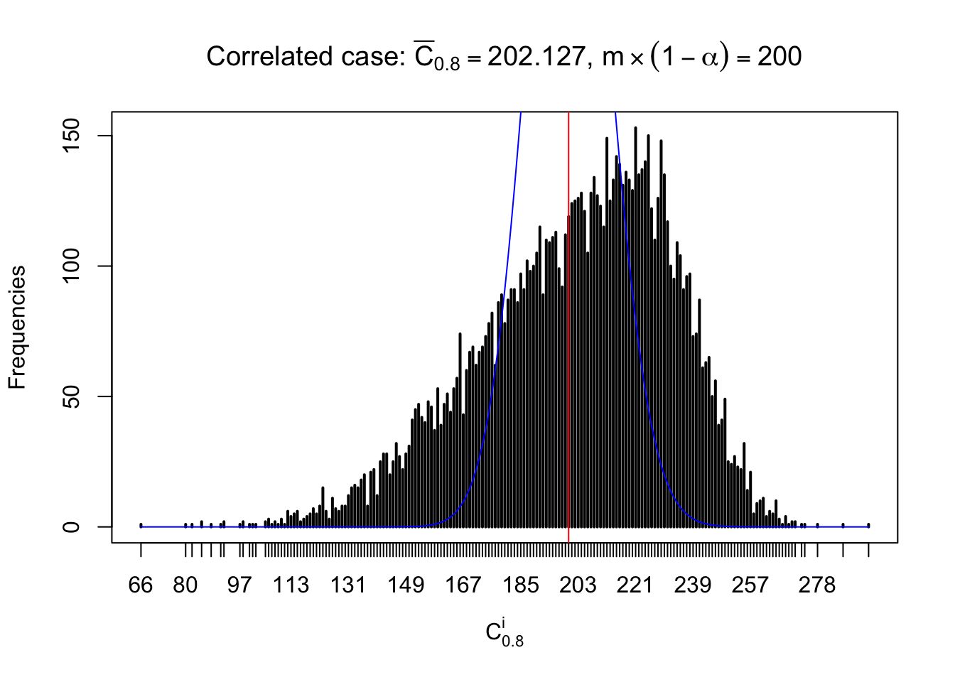
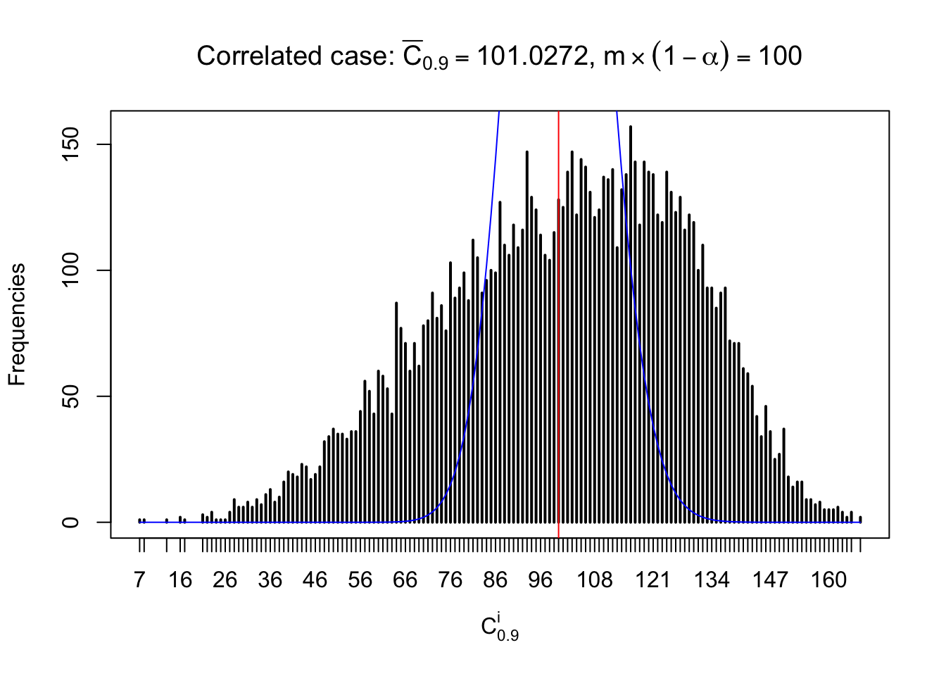
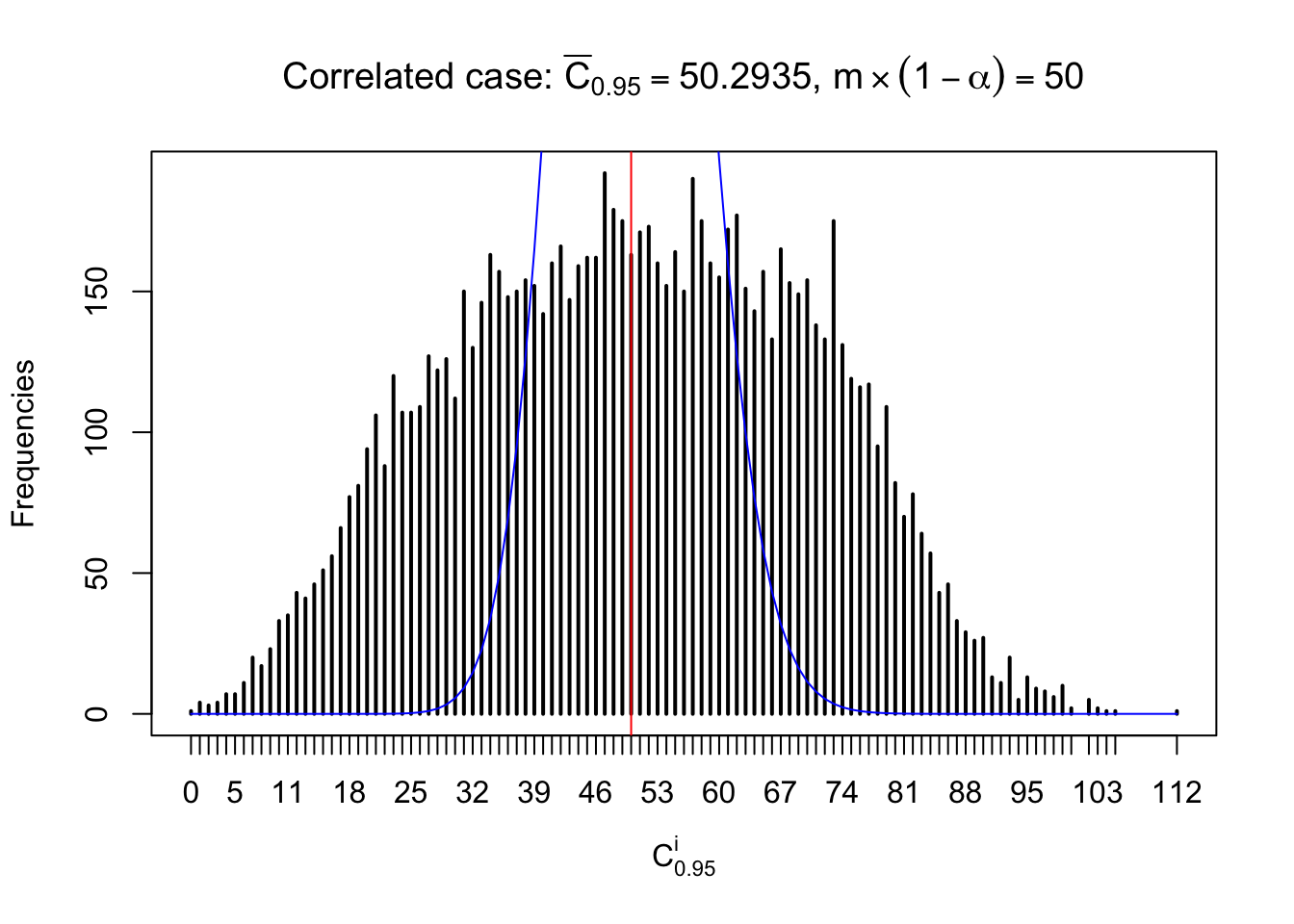
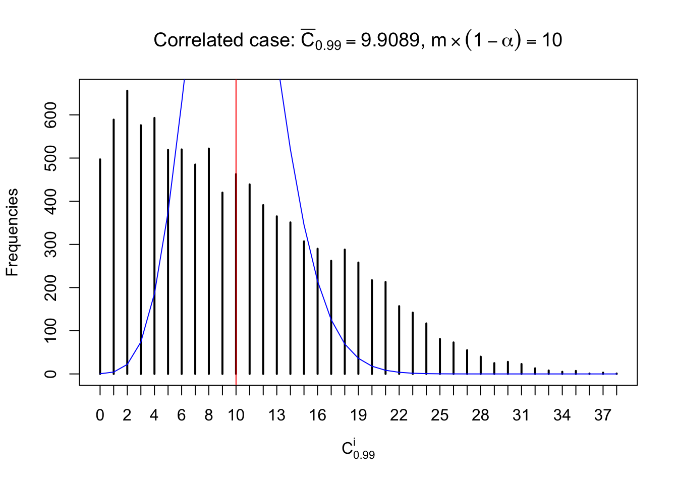
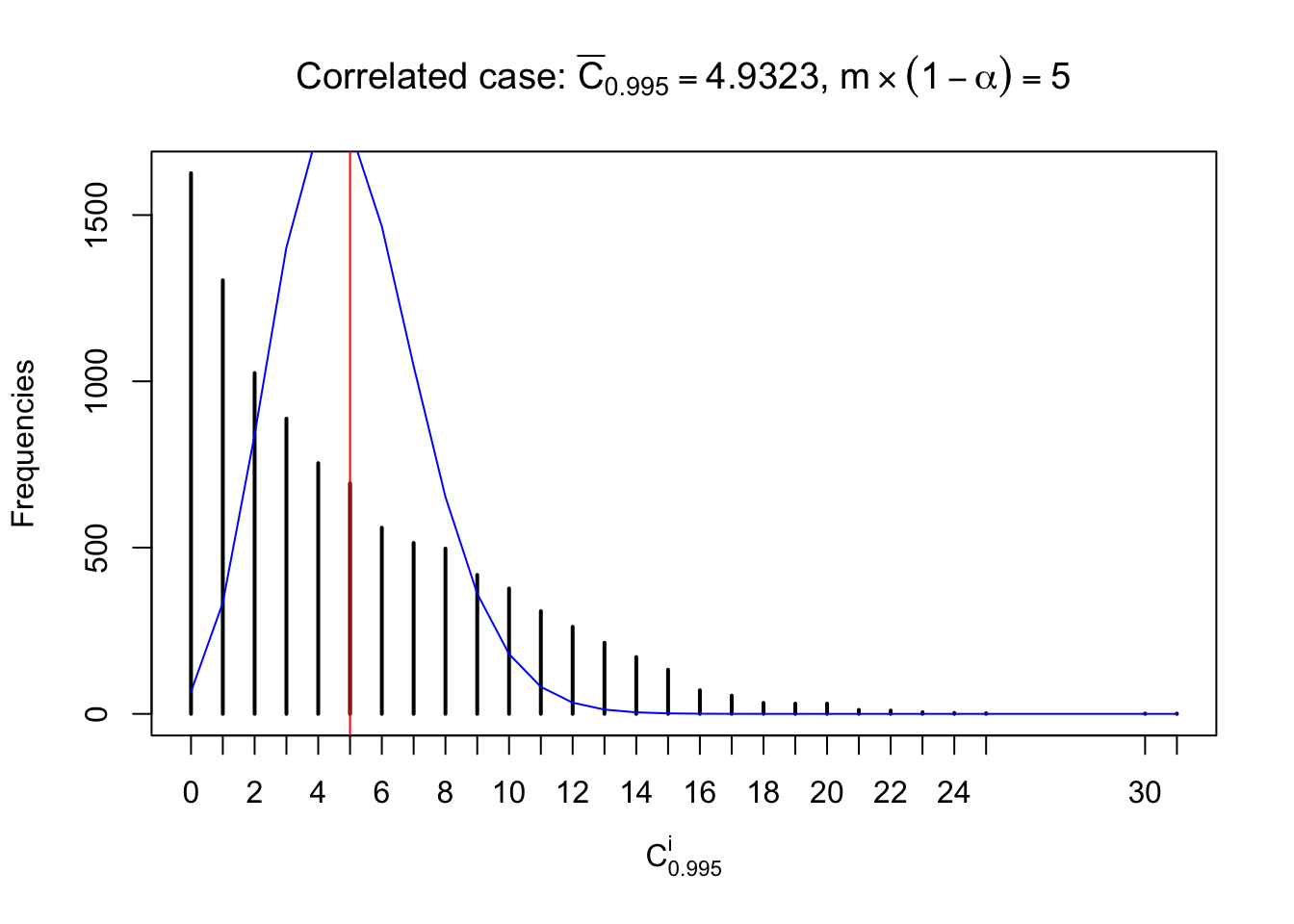
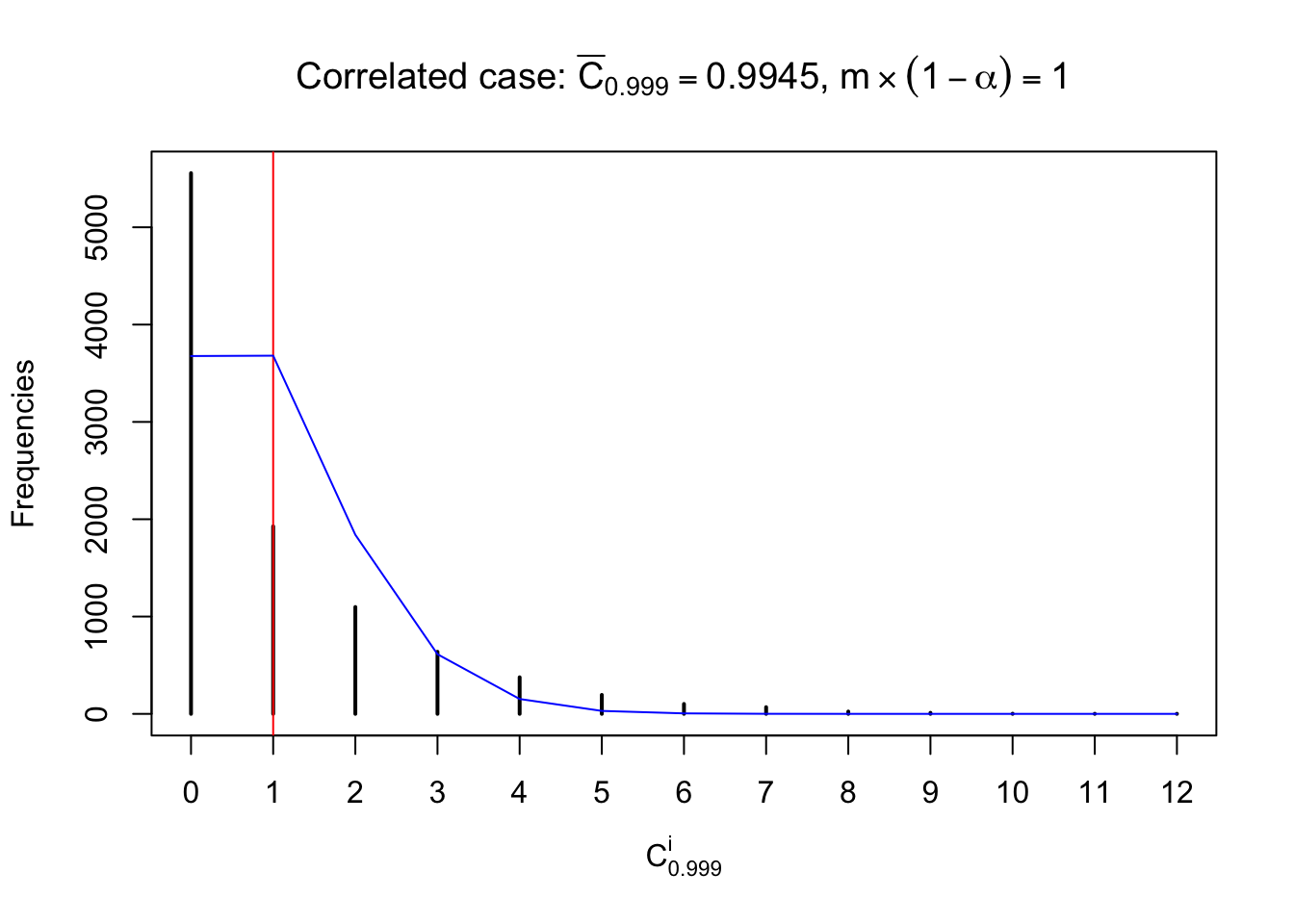
Each column of \(z\) should be seen as \(z\) scores of a non-differentially expressed gene in different data sets. Therefore, column-wise, the empirical distribution \(F_m^{C_j}\left(z\right)\) should be closer to \(\Phi\left(z\right)\) than \(F_m^{R_i}\left(z\right)\).
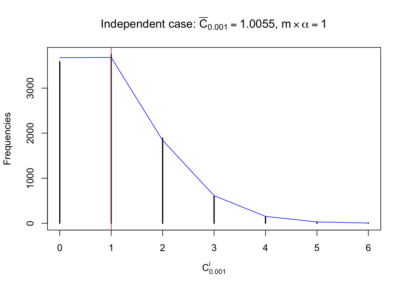
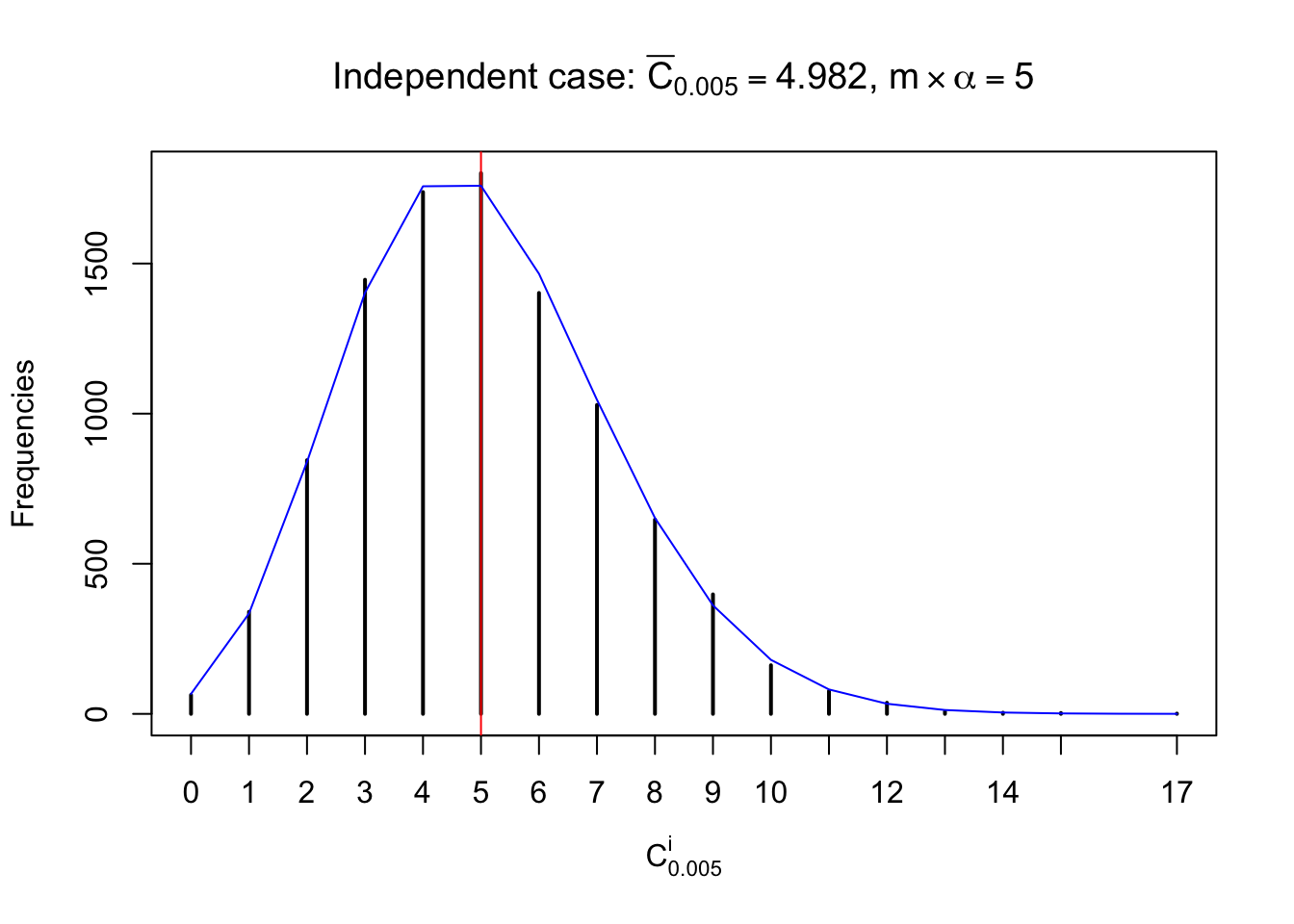
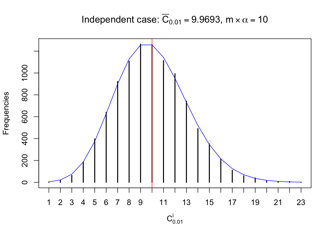
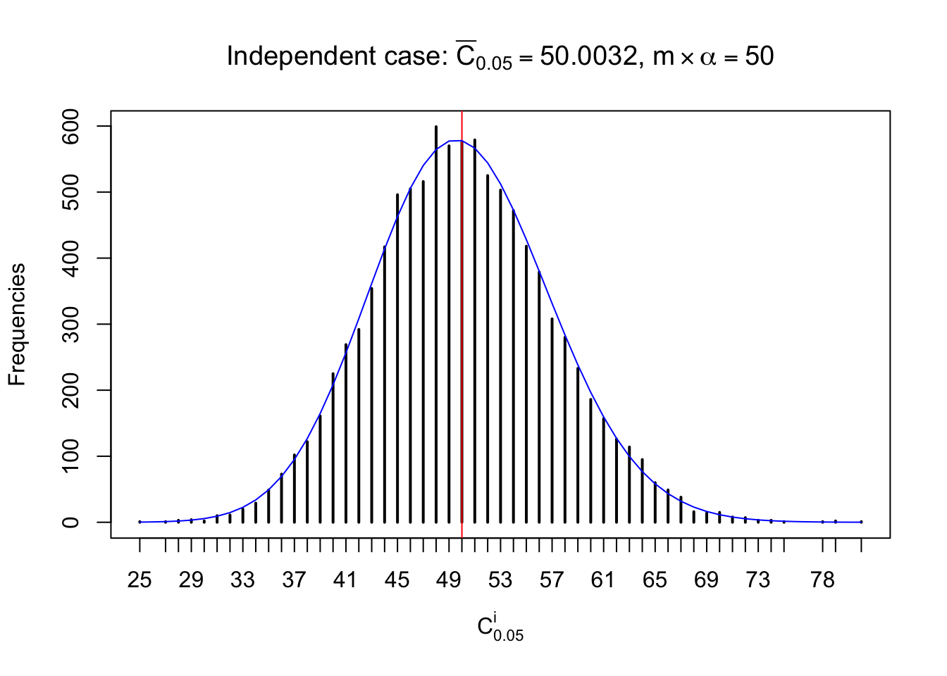
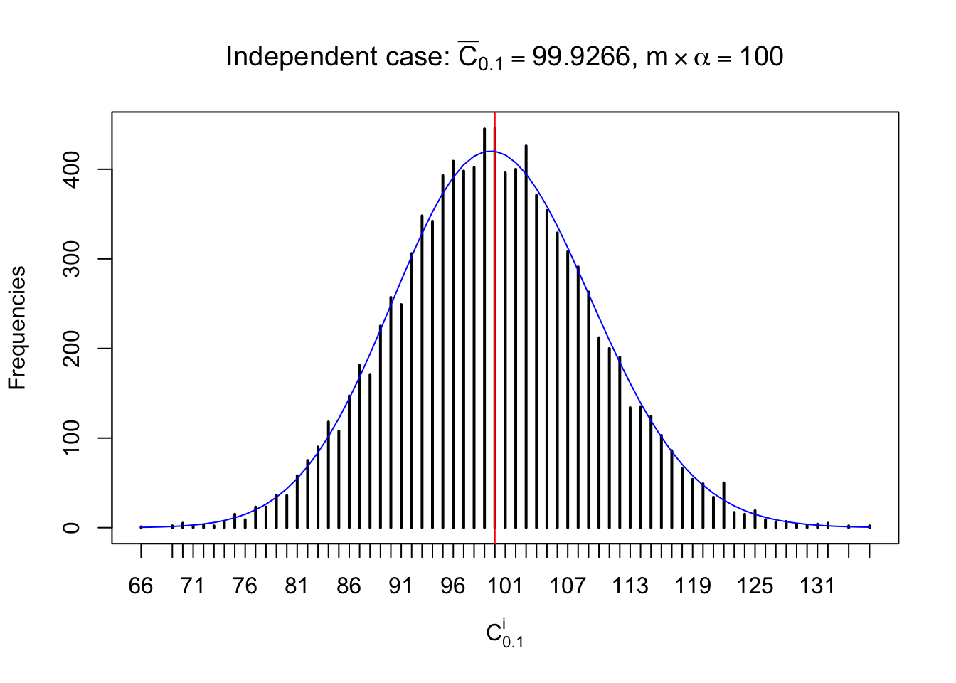
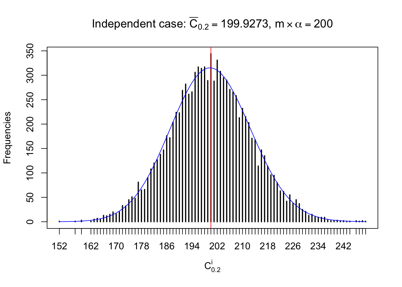
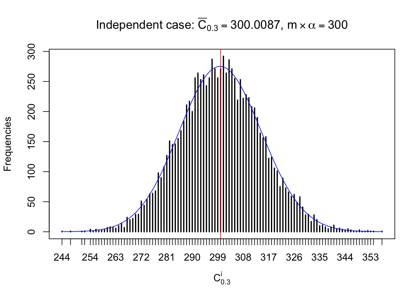
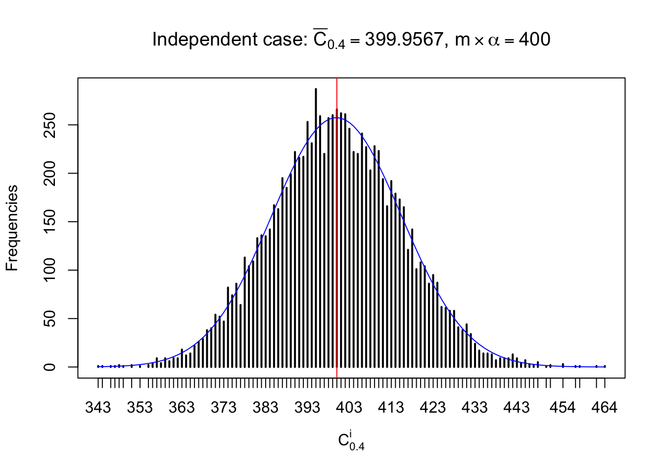
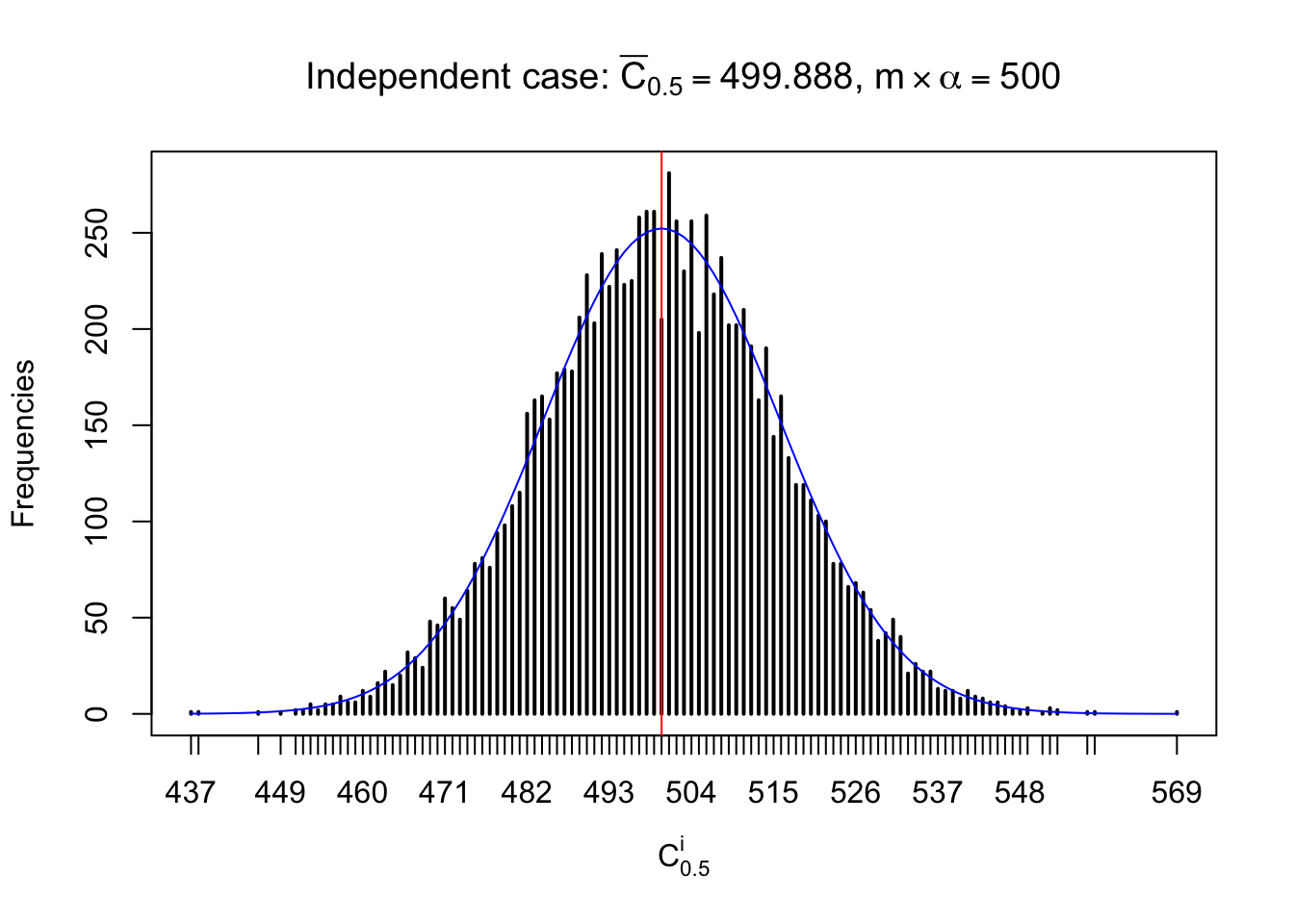
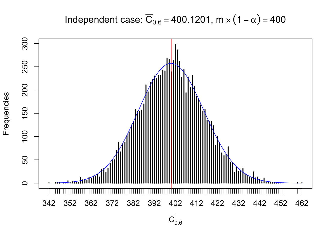
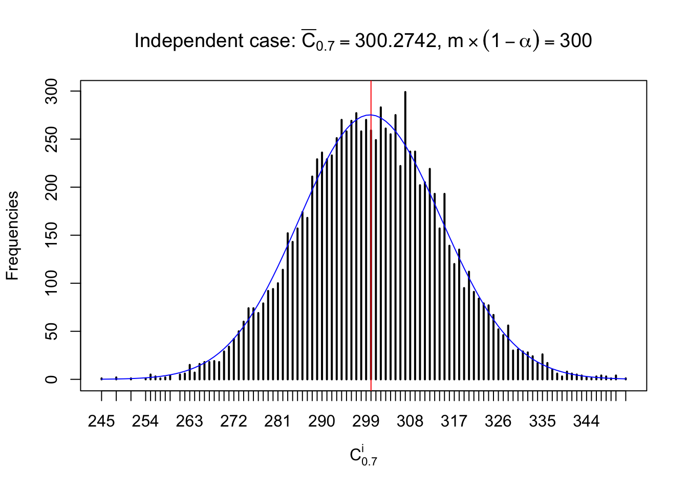
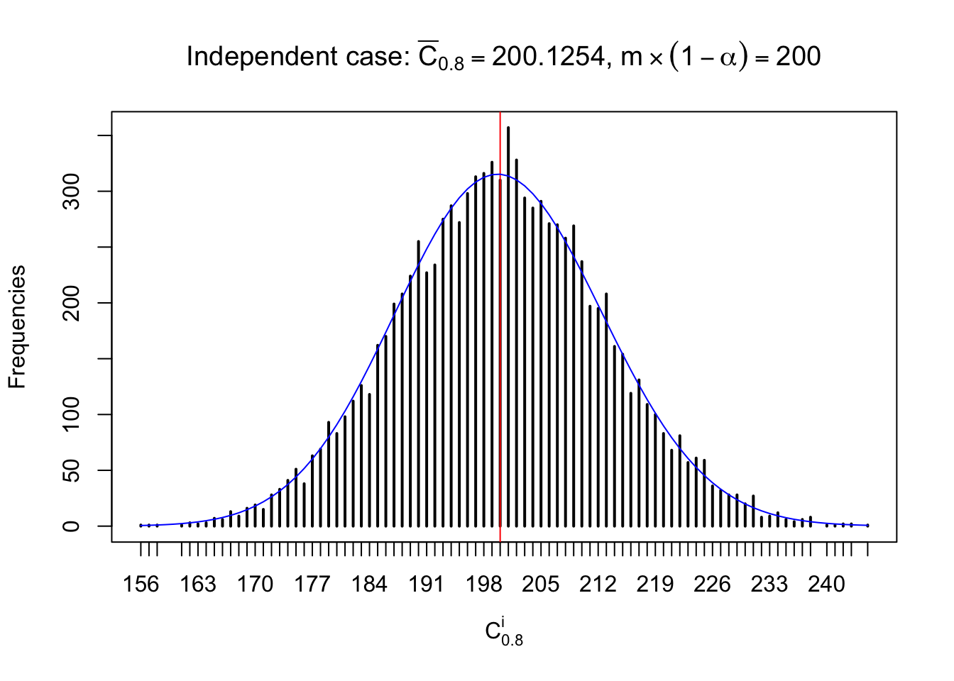
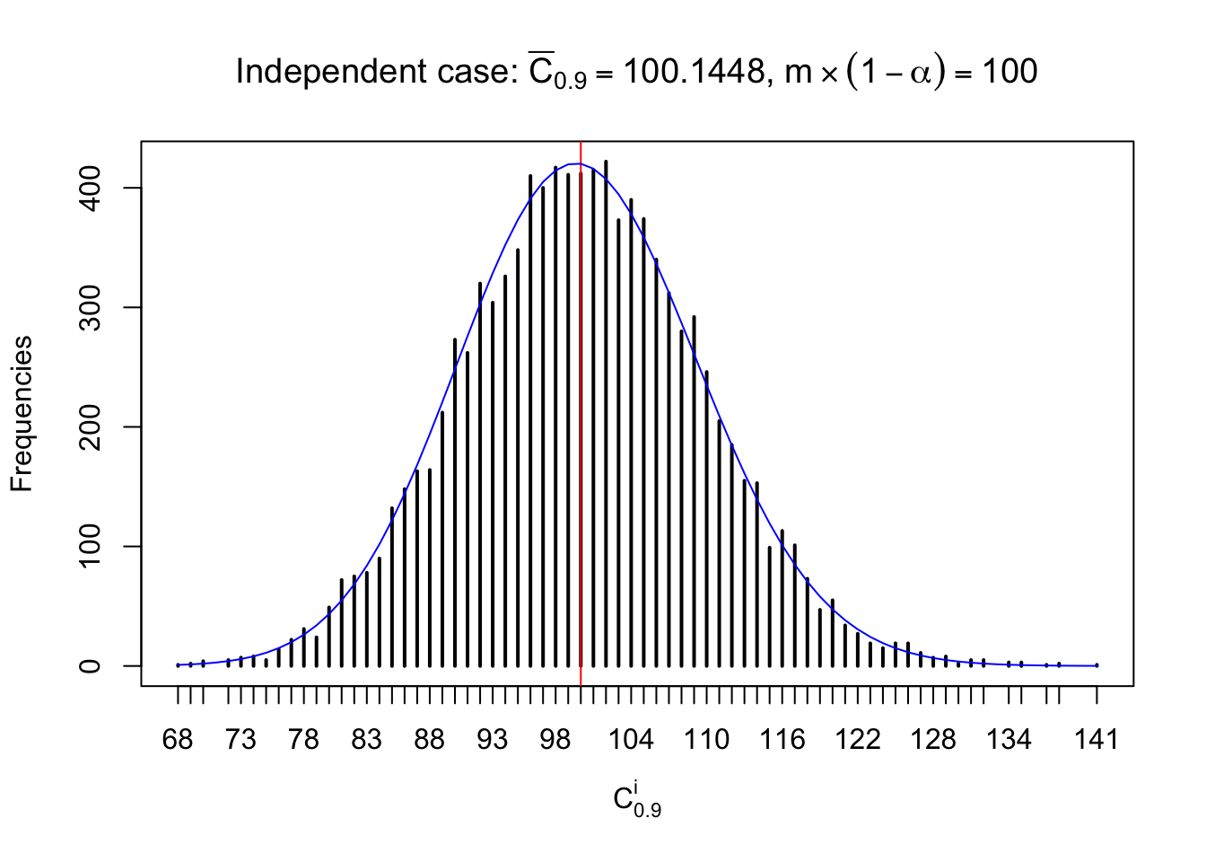
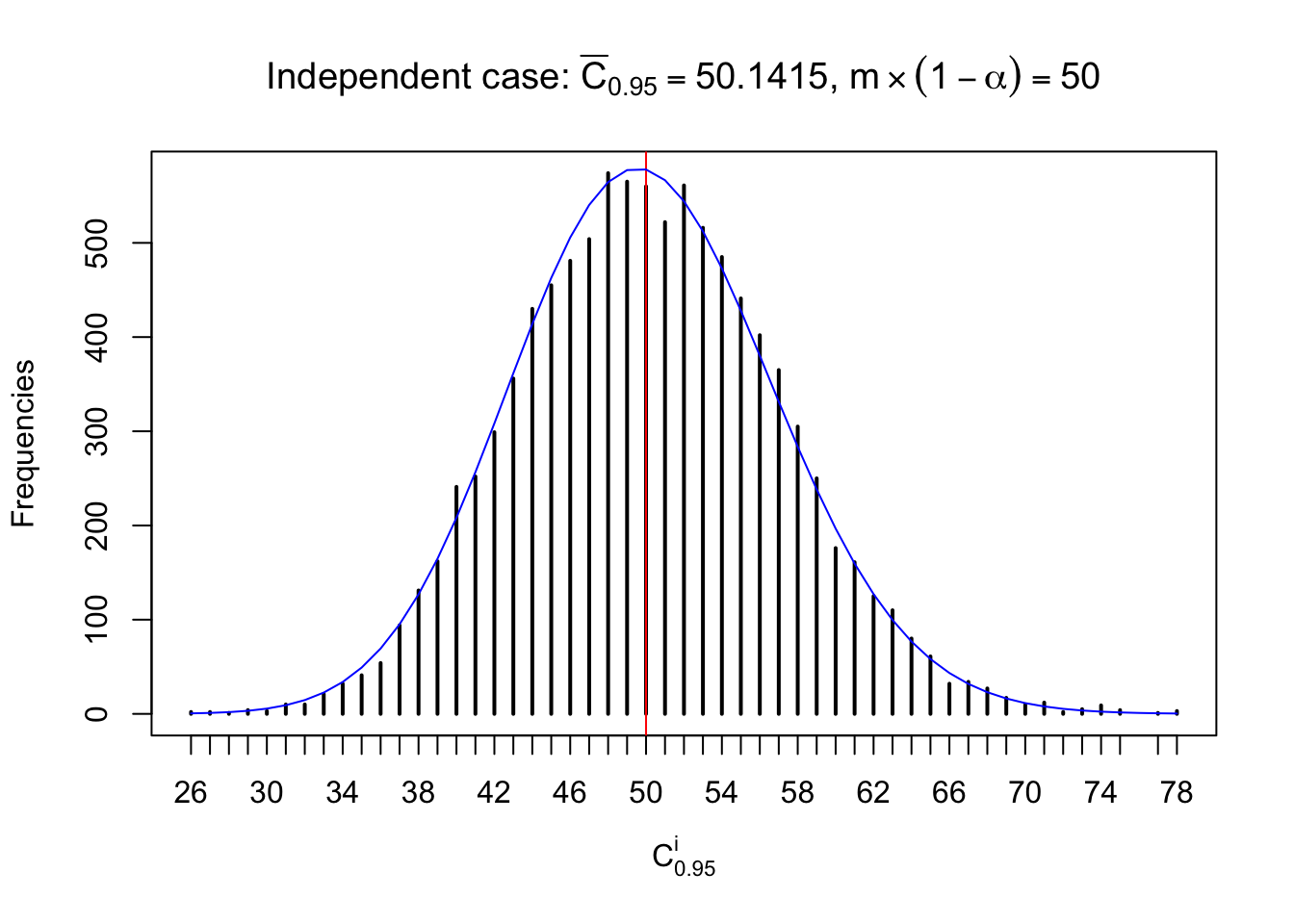
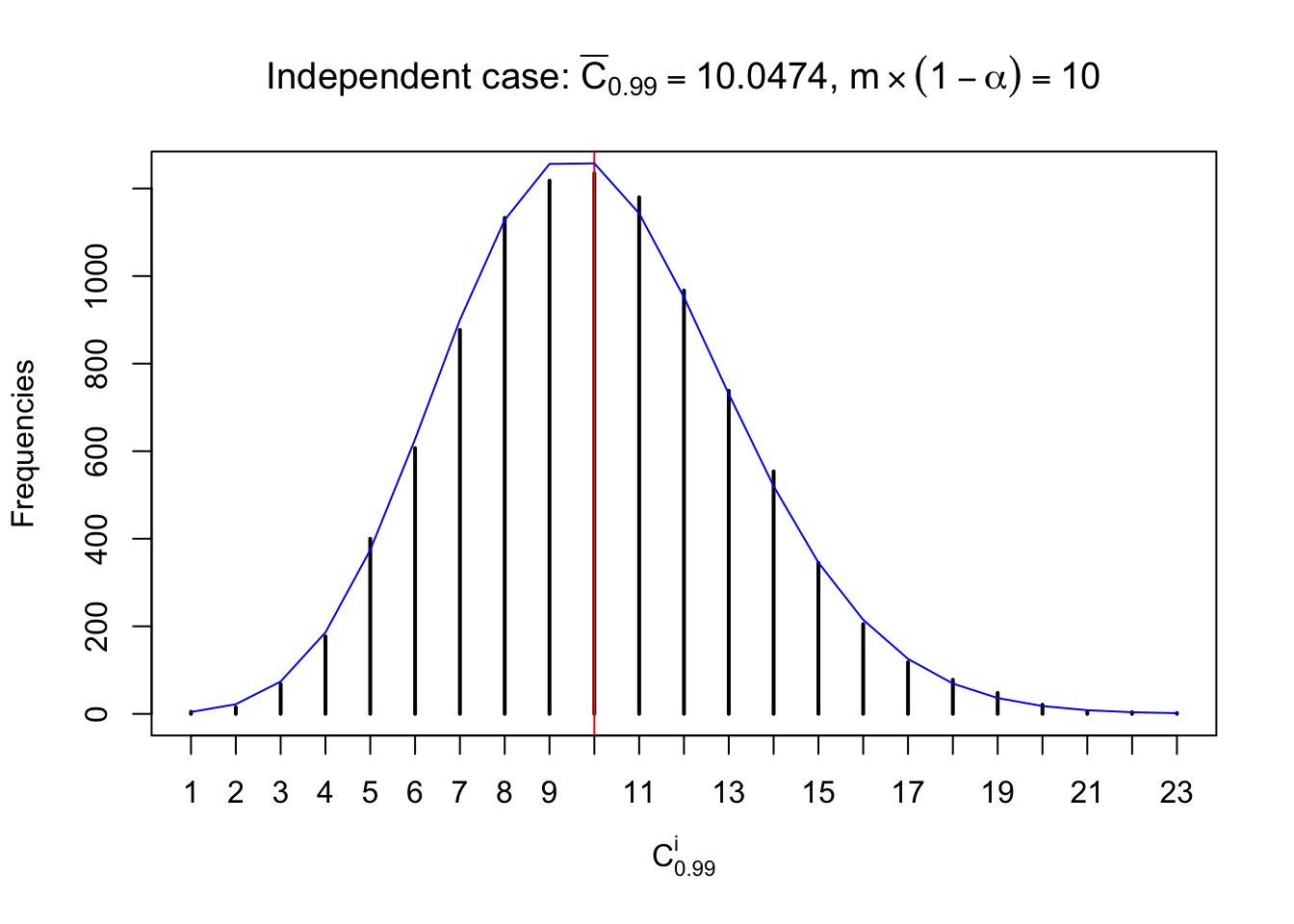
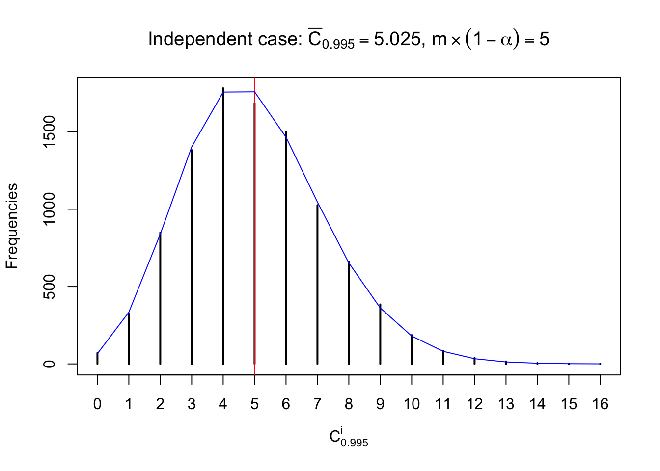
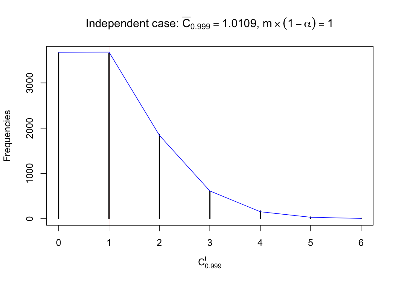
Similarly, we are plotting \(C_\alpha^i\), compared with their theoretical frequencies as follows.
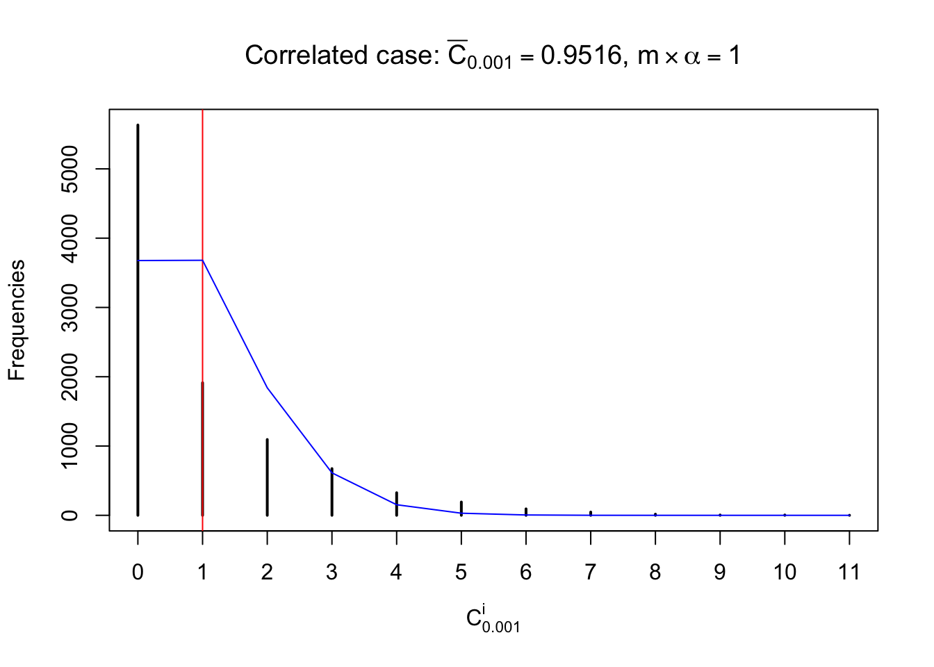
Independent case: column wise
Conclusion
The empirical distribution and the indicated marginal distribution of the correlated null \(z\) scores are behaving not different from the expectation.
Row-wise, the number of tail observations averages to what would be expected from correlated marginally \(N\left(0, 1\right)\) random samples, validating Prof. Stein’s intuition.
Column-wise, the distribution of the number of tail observations is closer to normal, closer to what would be expected under corelated marginally \(N\left(0, 1\right)\). Moreover, the distribution seems unimodal, and peaked at \(m\alpha\) when \(\alpha \leq0.5\) or \(m\left(1-\alpha\right)\) when \(\alpha\geq0.5\). It suggests that the marginal distribution of the null \(z\) scores for a certain gene is usually centered at \(0\), and more often than not, close to \(N\left(0, 1\right)\).
Session information
sessionInfo()R version 3.4.3 (2017-11-30)
Platform: x86_64-apple-darwin15.6.0 (64-bit)
Running under: macOS High Sierra 10.13.2
Matrix products: default
BLAS: /Library/Frameworks/R.framework/Versions/3.4/Resources/lib/libRblas.0.dylib
LAPACK: /Library/Frameworks/R.framework/Versions/3.4/Resources/lib/libRlapack.dylib
locale:
[1] en_US.UTF-8/en_US.UTF-8/en_US.UTF-8/C/en_US.UTF-8/en_US.UTF-8
attached base packages:
[1] stats graphics grDevices utils datasets methods base
loaded via a namespace (and not attached):
[1] compiler_3.4.3 backports_1.1.2 magrittr_1.5 rprojroot_1.3-1
[5] tools_3.4.3 htmltools_0.3.6 yaml_2.1.16 Rcpp_0.12.14
[9] stringi_1.1.6 rmarkdown_1.8 knitr_1.17 git2r_0.20.0
[13] stringr_1.2.0 digest_0.6.13 evaluate_0.10.1This R Markdown site was created with workflowr