Knockoff on Small Signals
Lei Sun
2018-02-05
Last updated: 2018-04-03
Code version: 5bce84a
Introduction
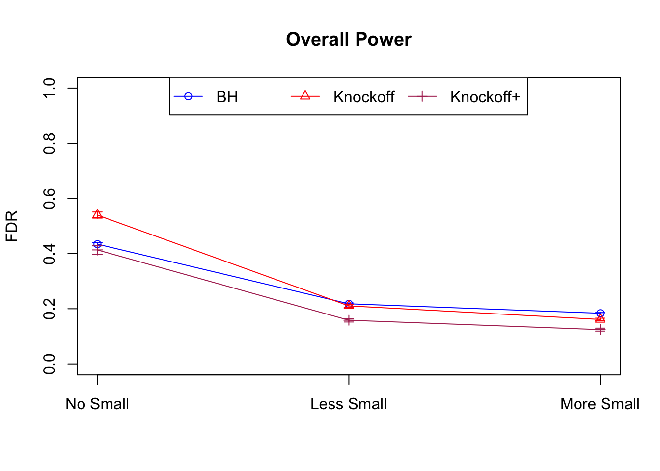
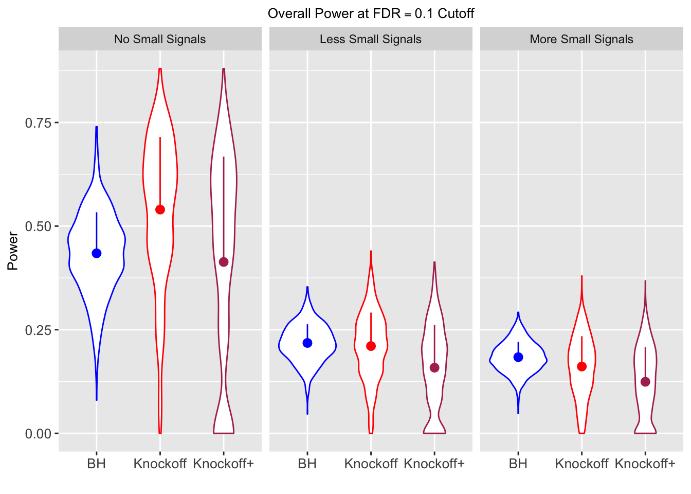
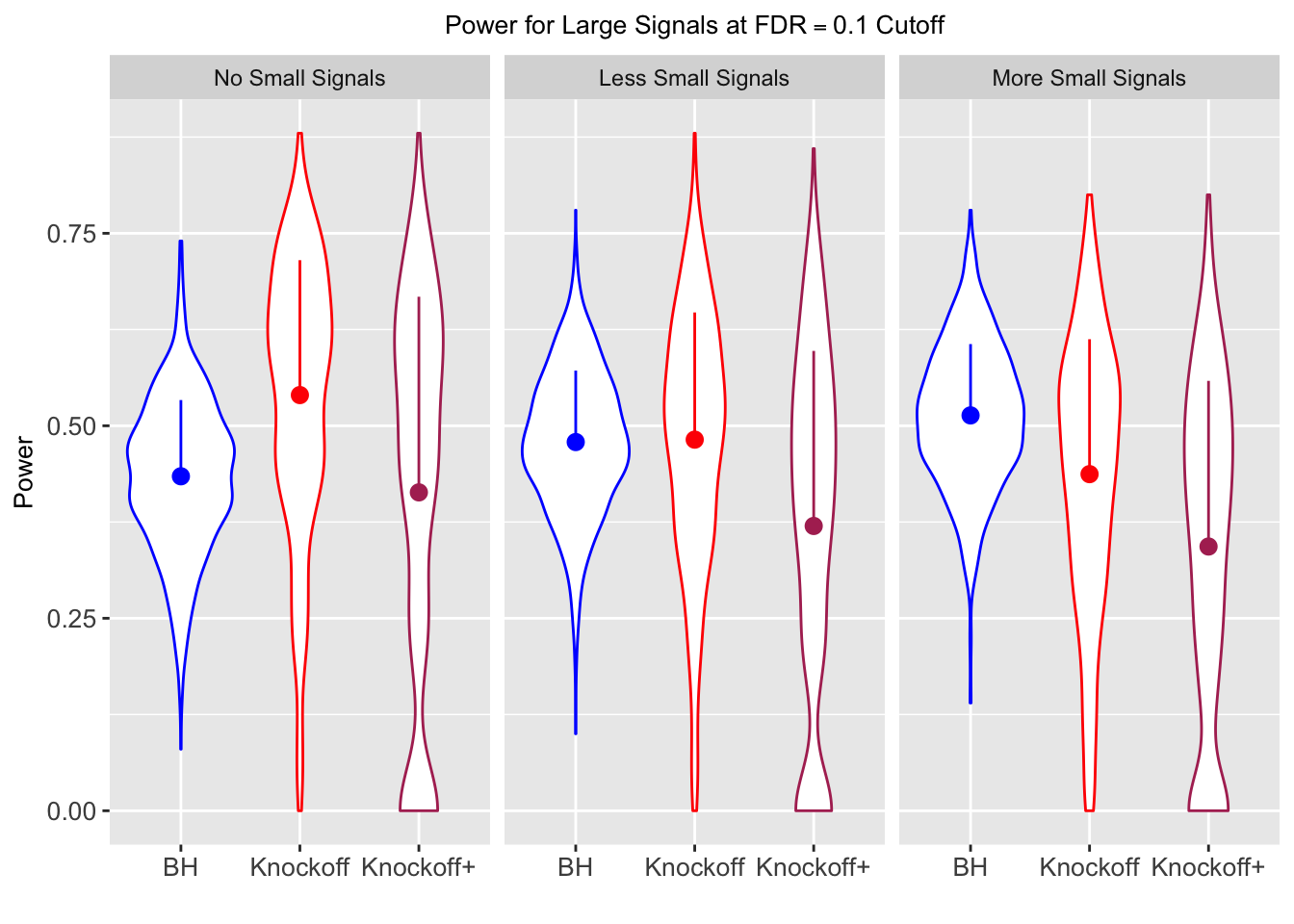
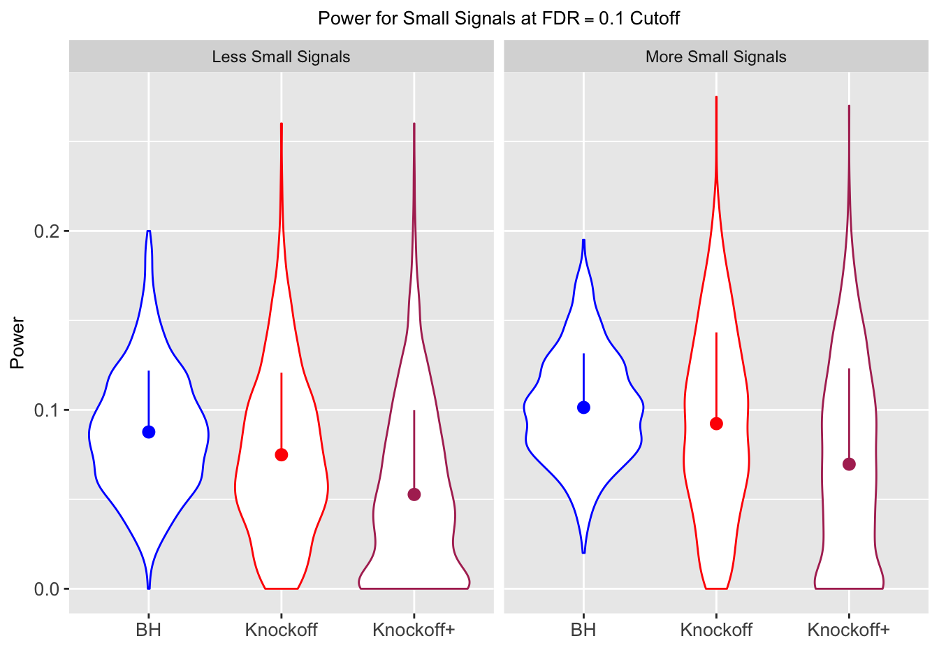
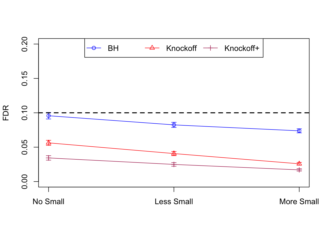
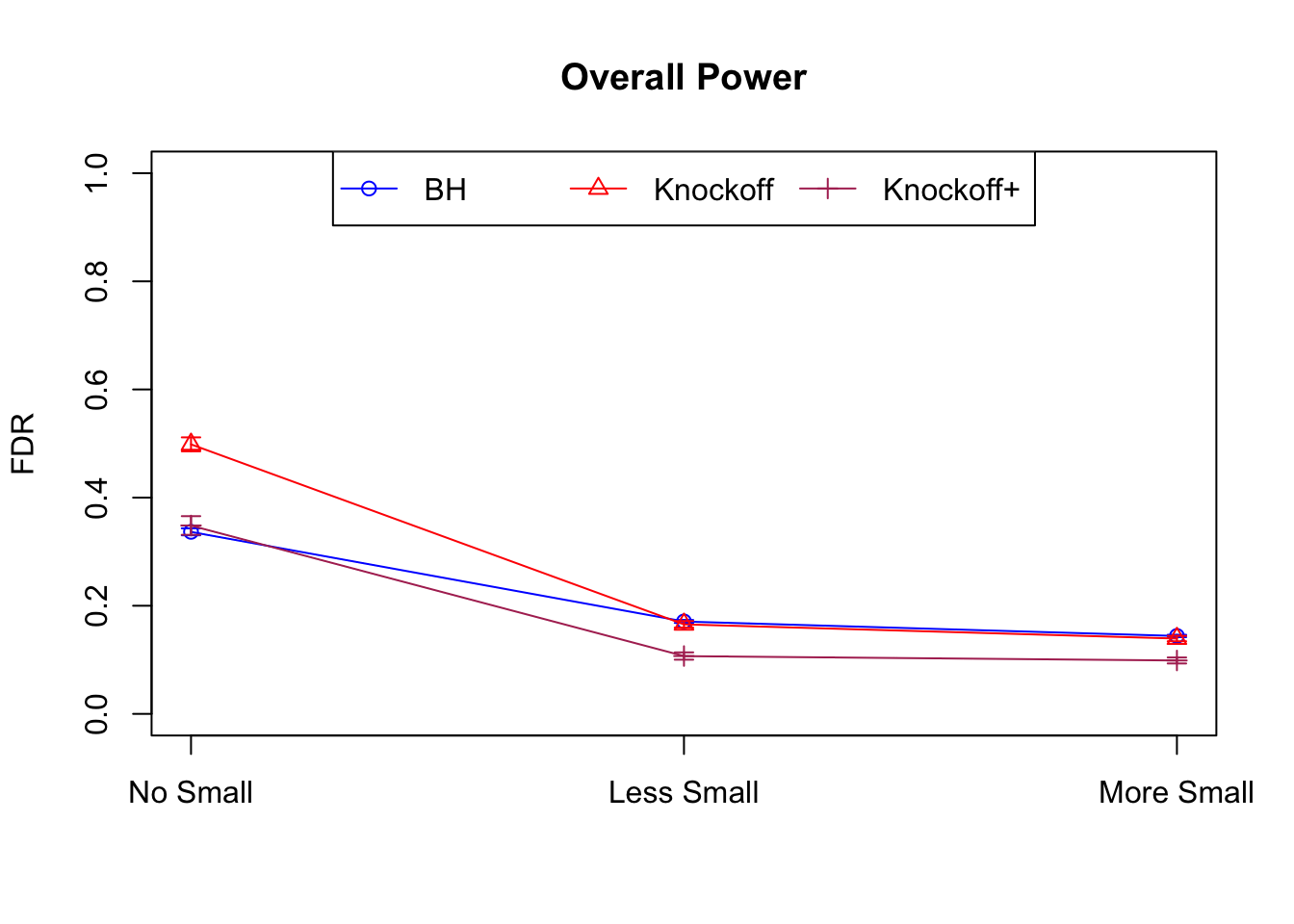
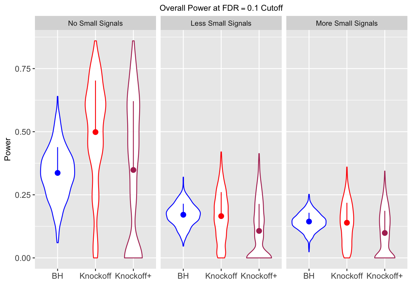
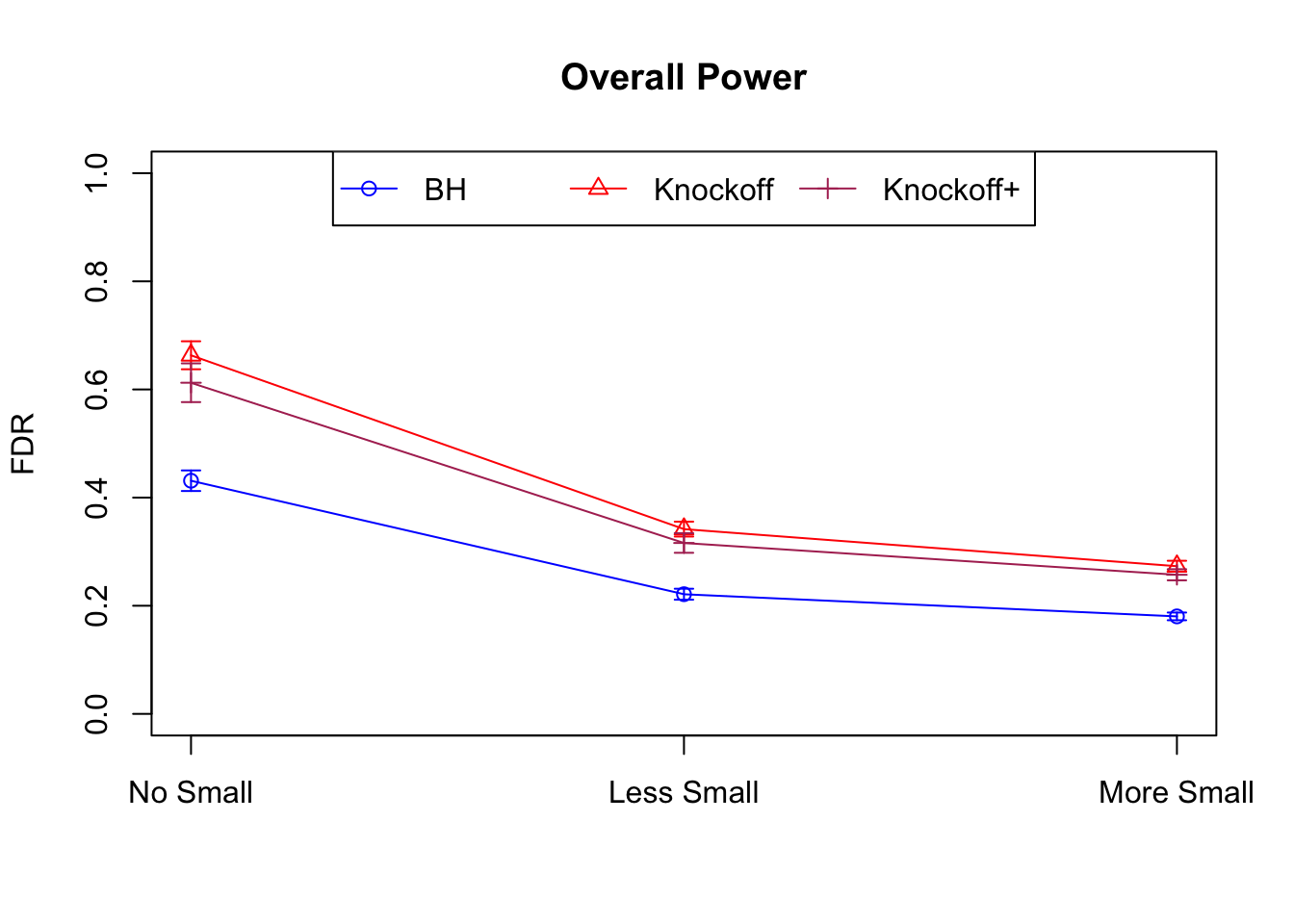
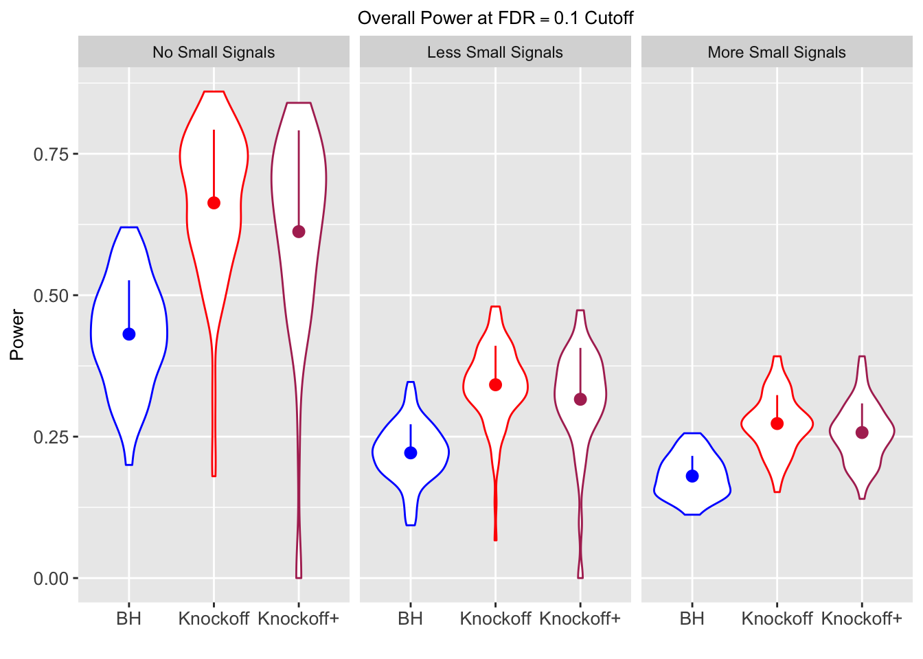
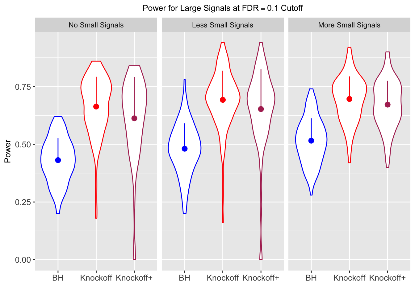
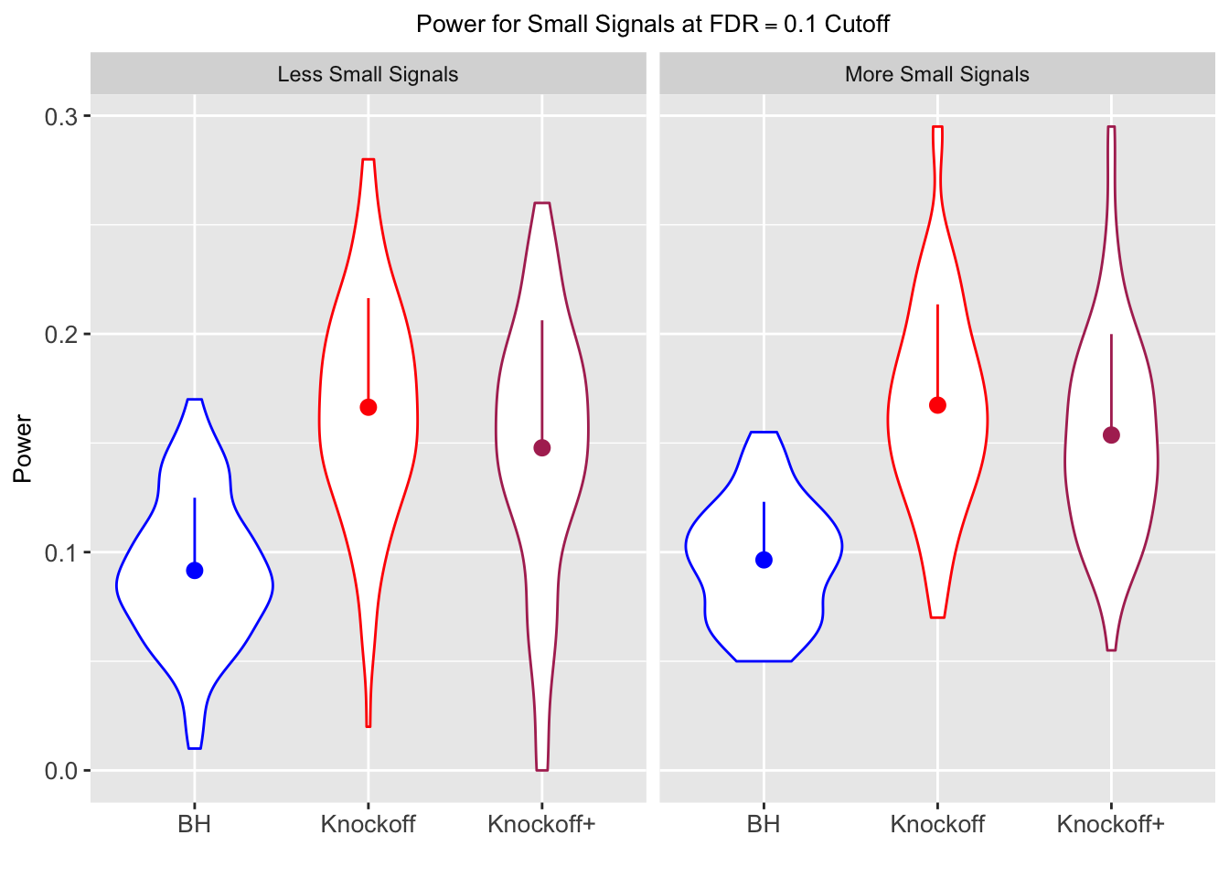
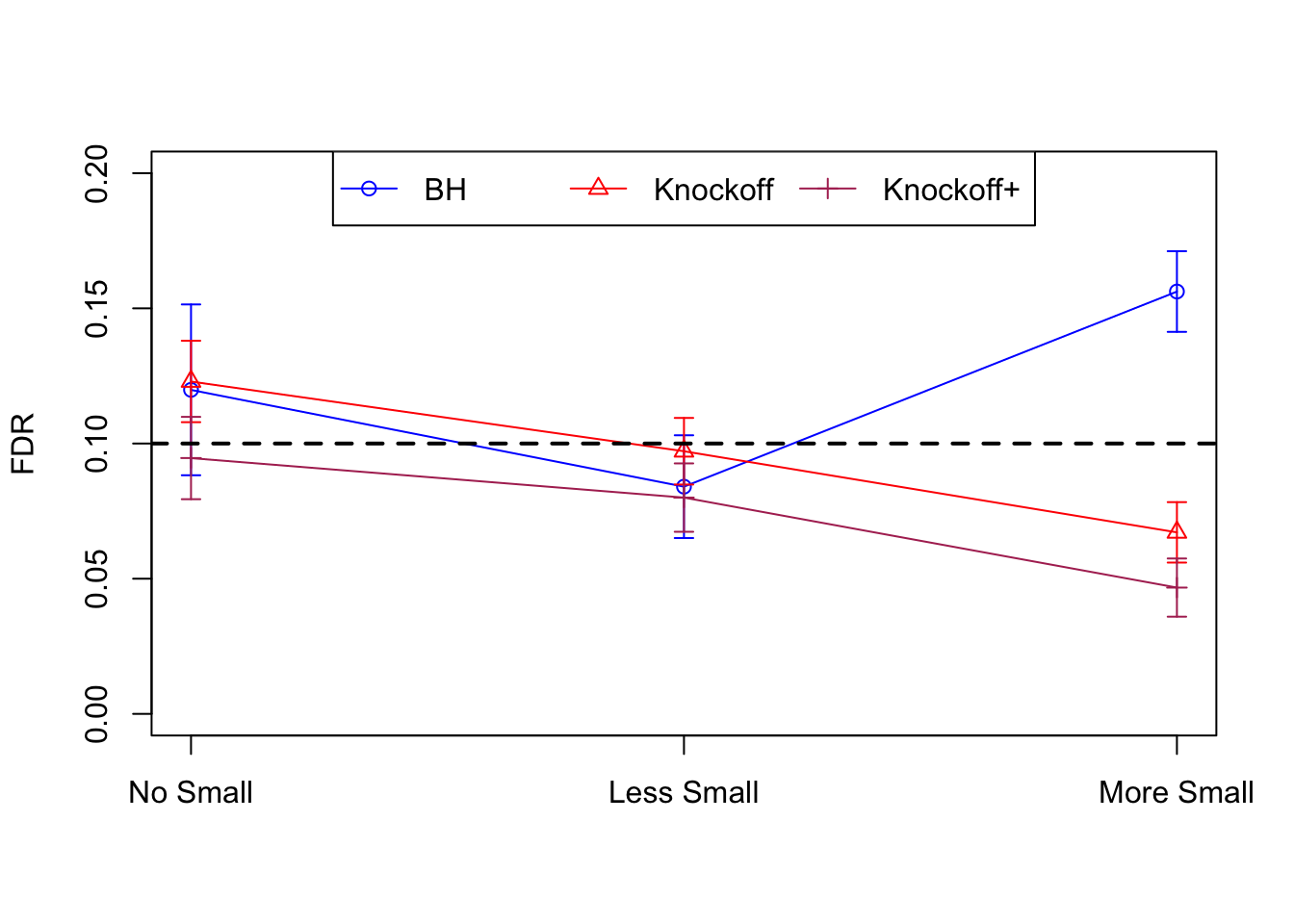
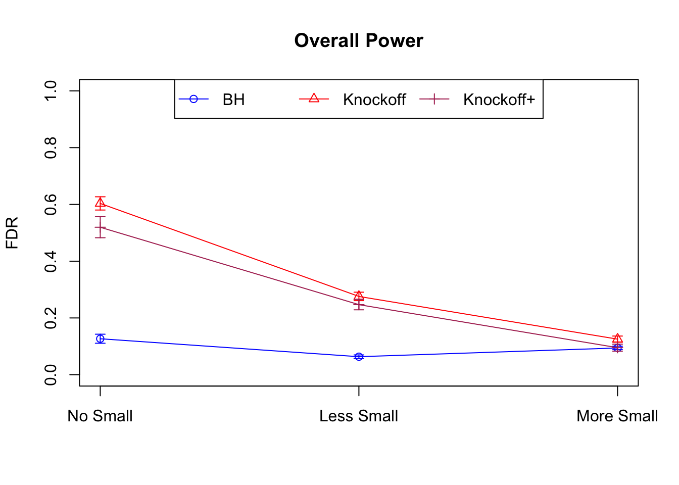
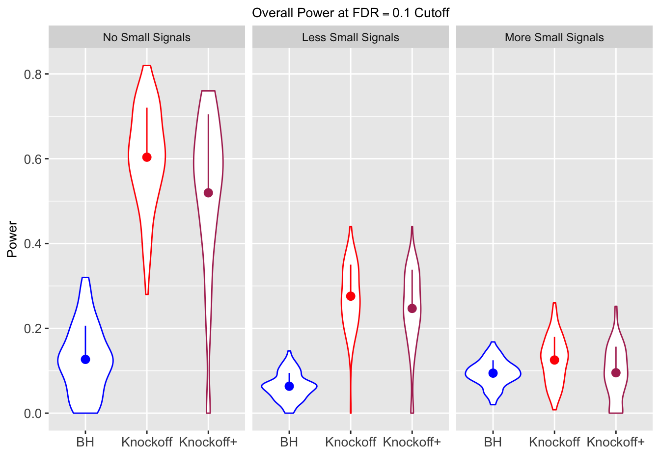
In the Knockoff paper simulations, \(\beta\)’s are either \(0\) or \(A\). Here we are replicating the results, and investigating how well Knockoff deal with small signals.
In the following simulations, we always have \(n = 3000\), \(p = 1000\), For a certain \(\beta\), \(Y_n \sim N(X_{n\times p}\beta_p, I_n)\). Out of \(p = 1000\) \(\beta_j\)’s, here are three scenarios.
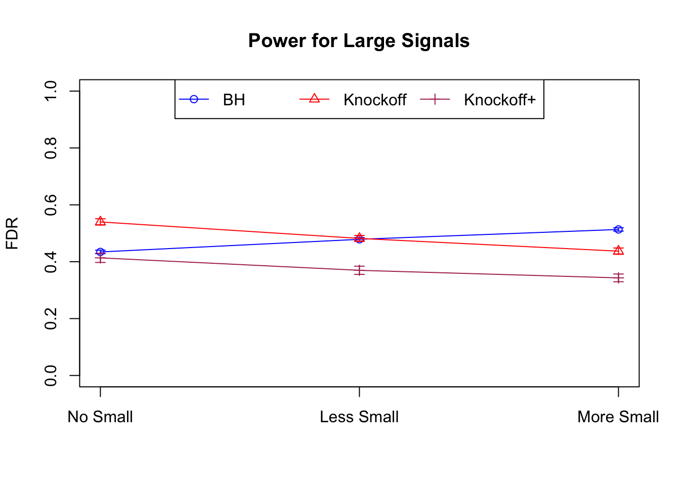
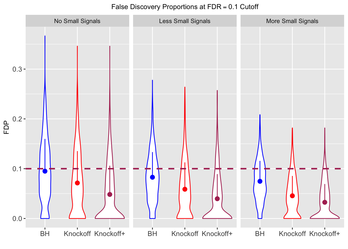
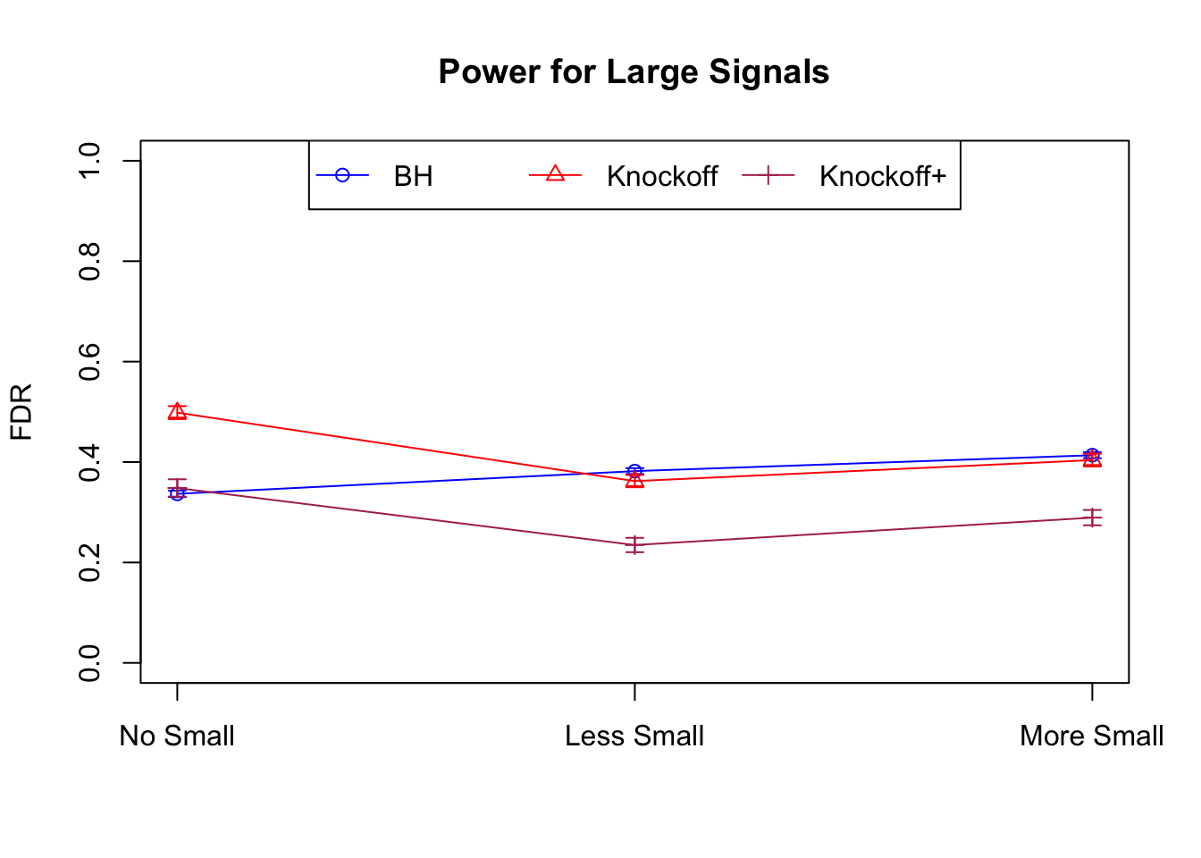
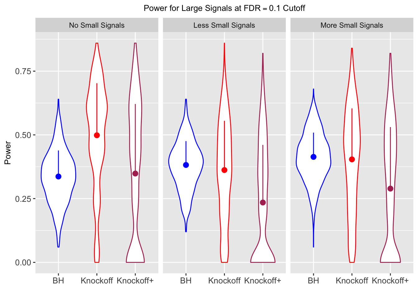
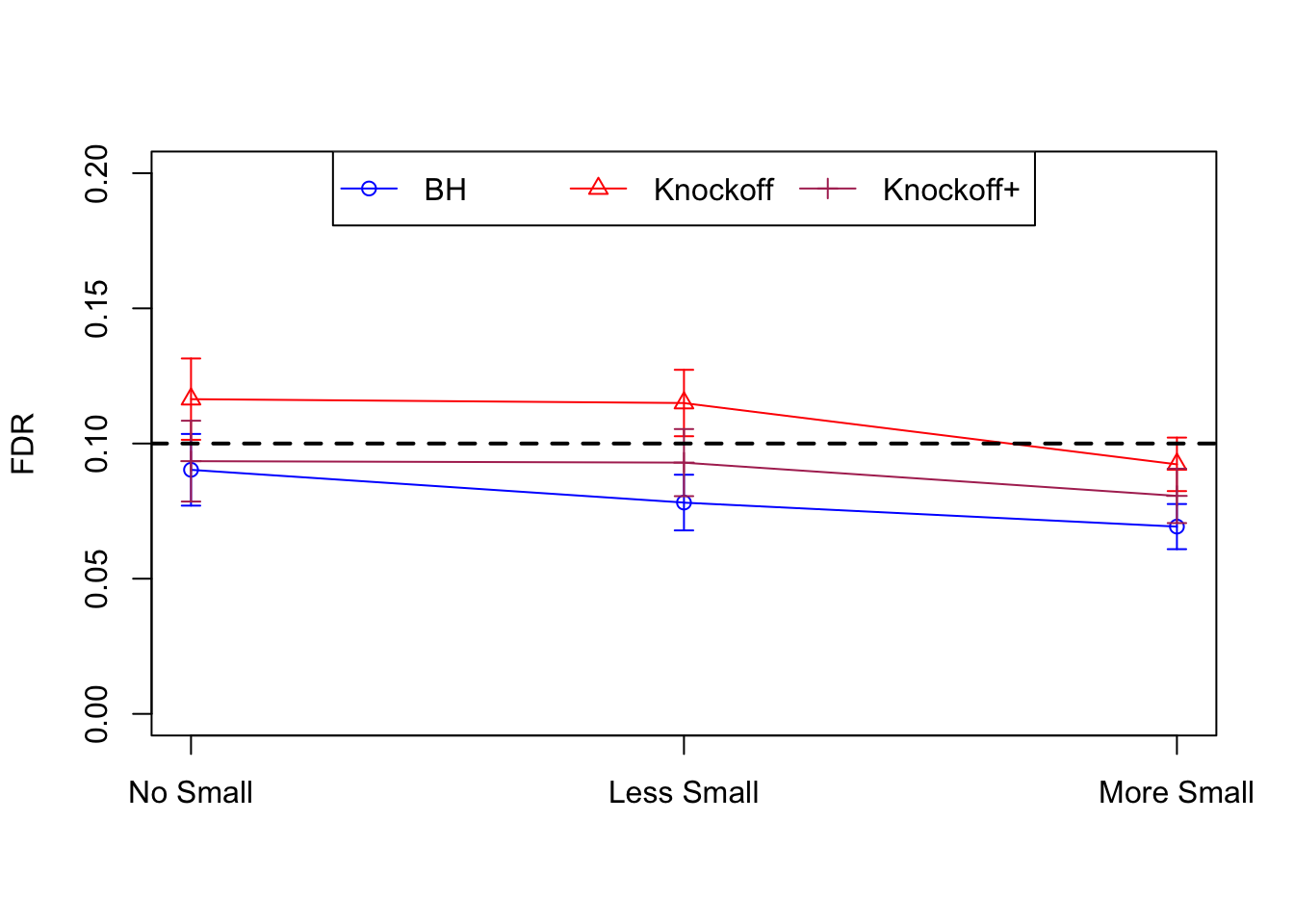
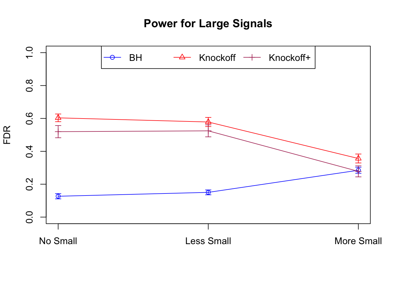
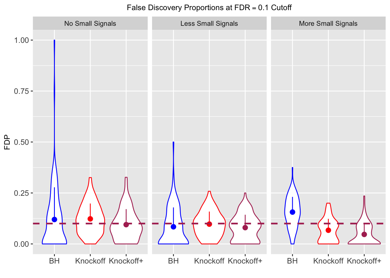
- Scenario 1: \(950\) are 0, and the rest \(50\) are \(A = 3.5\). (replicating a data point on Fig 3 of the
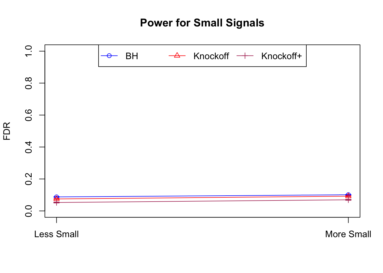
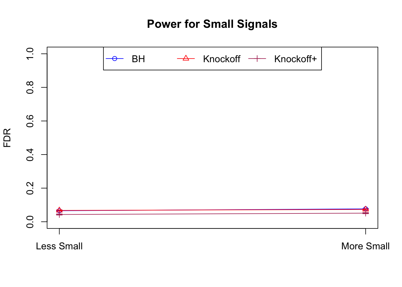
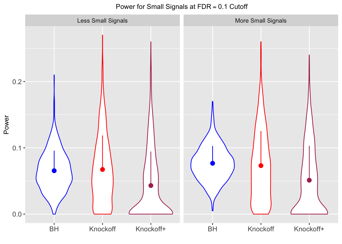
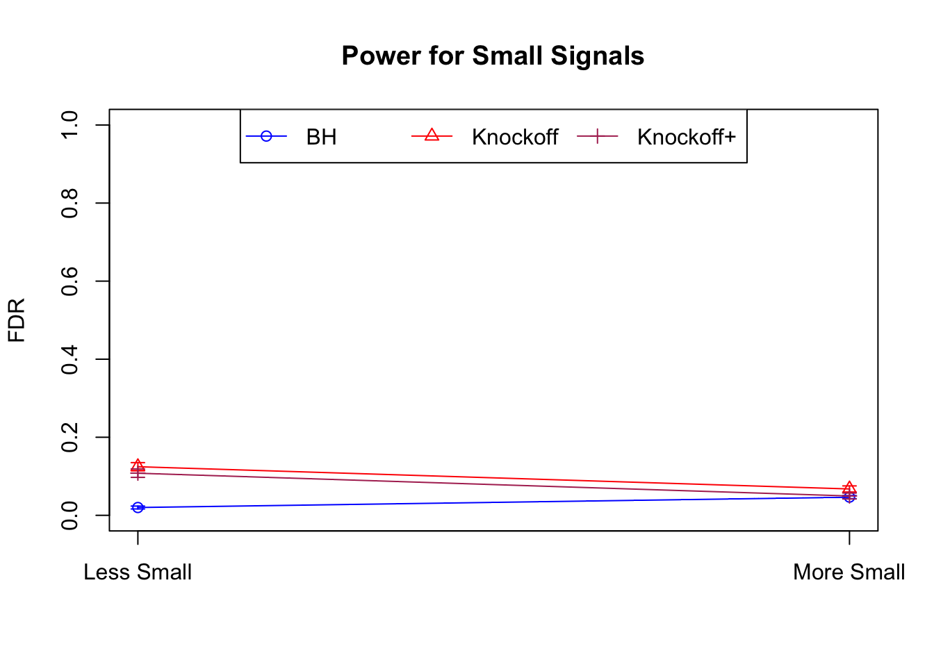
Knockoffpaper) - Scenario 2: \(850\) are 0, \(50\) are \(A = 3.5\) as large signals, and the rest \(100\) are small signals uniformly from \(0\) to \(3.5\).
- Scenario 3: \(750\) are 0, \(50\) are \(A = 3.5\) as large signals, and the rest \(200\) are small signals uniformly from \(0\) to \(3.5\).
Loading required package: foreachLoading required package: iteratorsLoading required package: paralleln <- 3000
p <- 1000
k <- 50
q <- 0.1
A <- 3.5Scenario 1: 50 large signals, no small signals, 950 zeroes.
X <- matrix(rnorm(n * p), n , p)
X <- svd(X)$u
Xk <- knockoff::create.fixed(X)
Xk <- Xk$Xk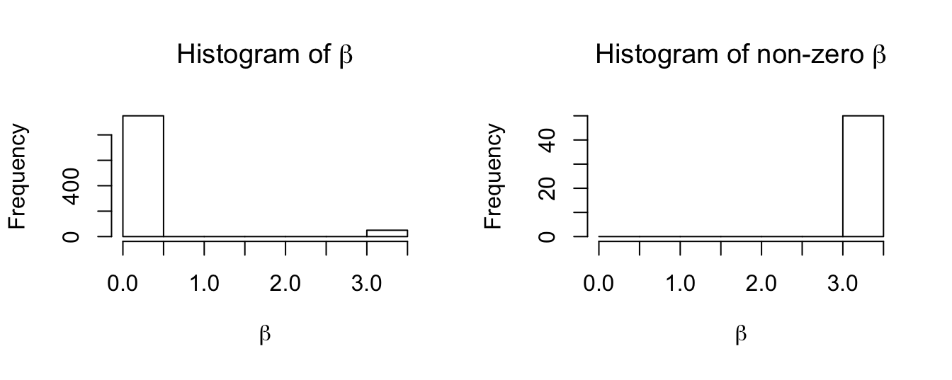
Scenario 2: 50 large signals, 100 small signals, 850 zeroes.
X <- matrix(rnorm(n * p), n , p)
X <- svd(X)$u
Xk <- knockoff::create.fixed(X)
Xk <- Xk$Xk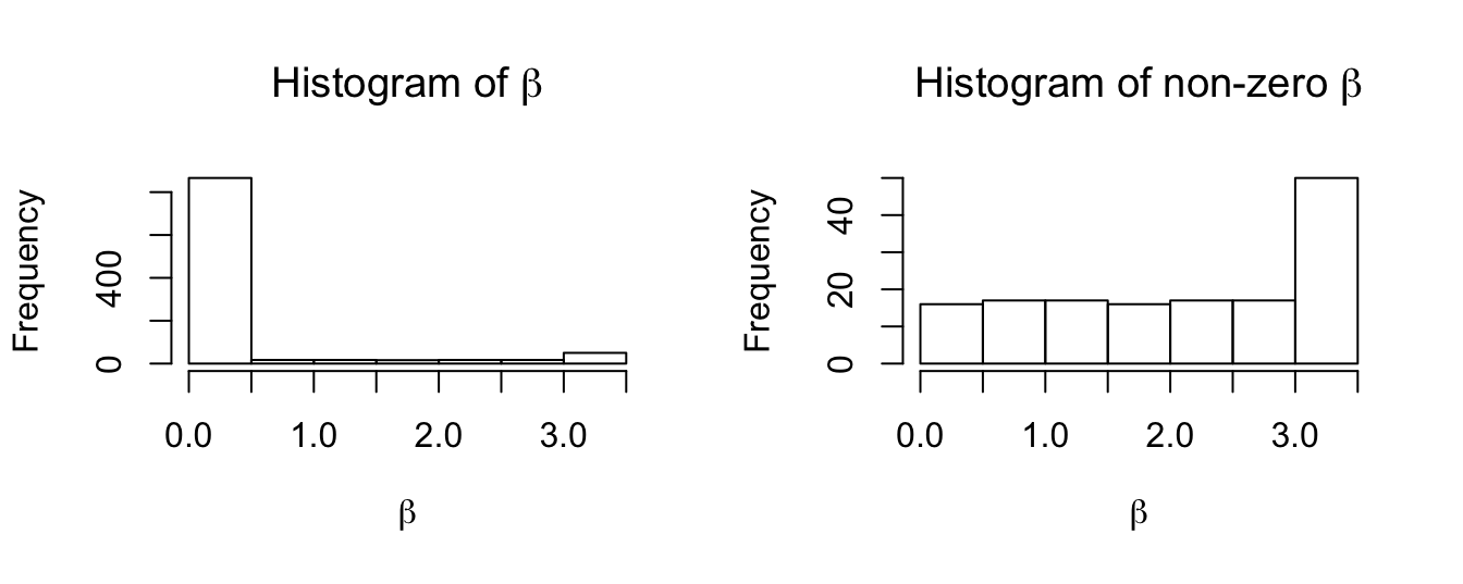
Scenario 3: 50 large signals, 200 small signals, 750 zeroes.
X <- matrix(rnorm(n * p), n , p)
X <- svd(X)$u
Xk <- knockoff::create.fixed(X)
Xk <- Xk$Xk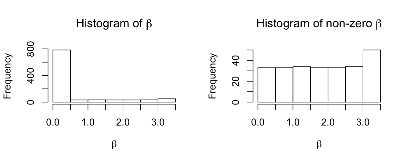
Fix-\(X\) Knockoffs
Orthogonal design
\(X\) has random orthonormal columns
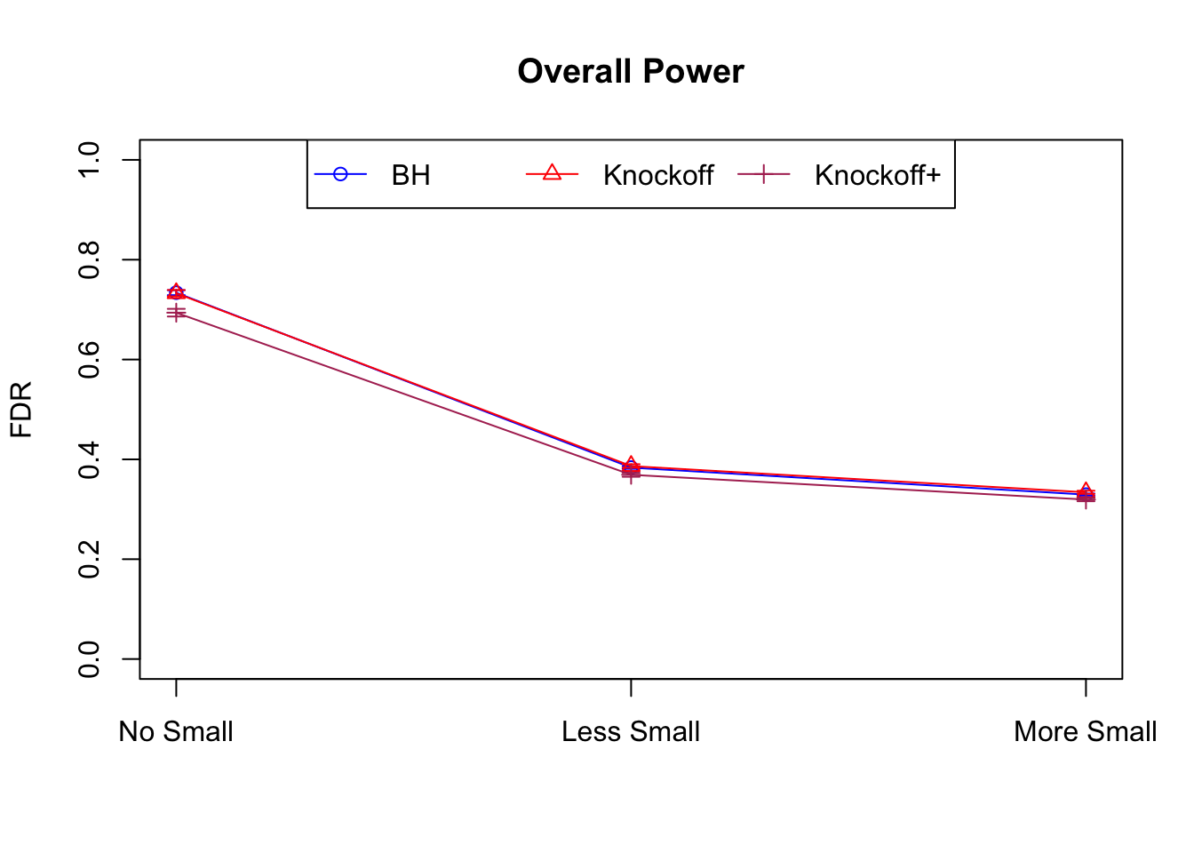
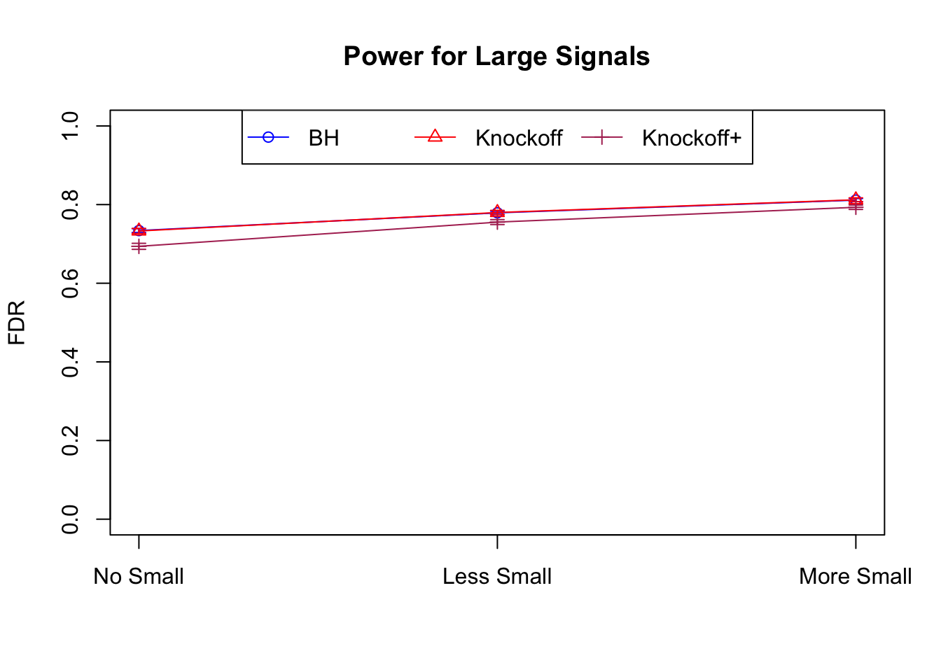
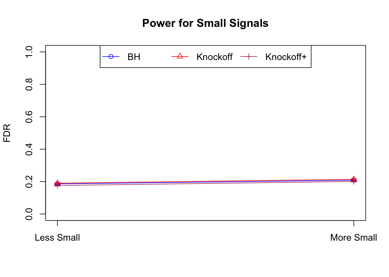
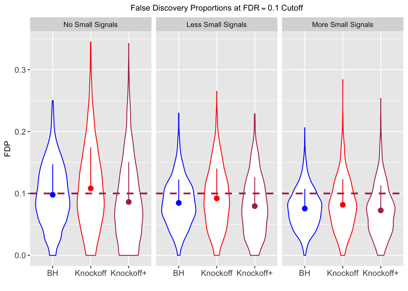
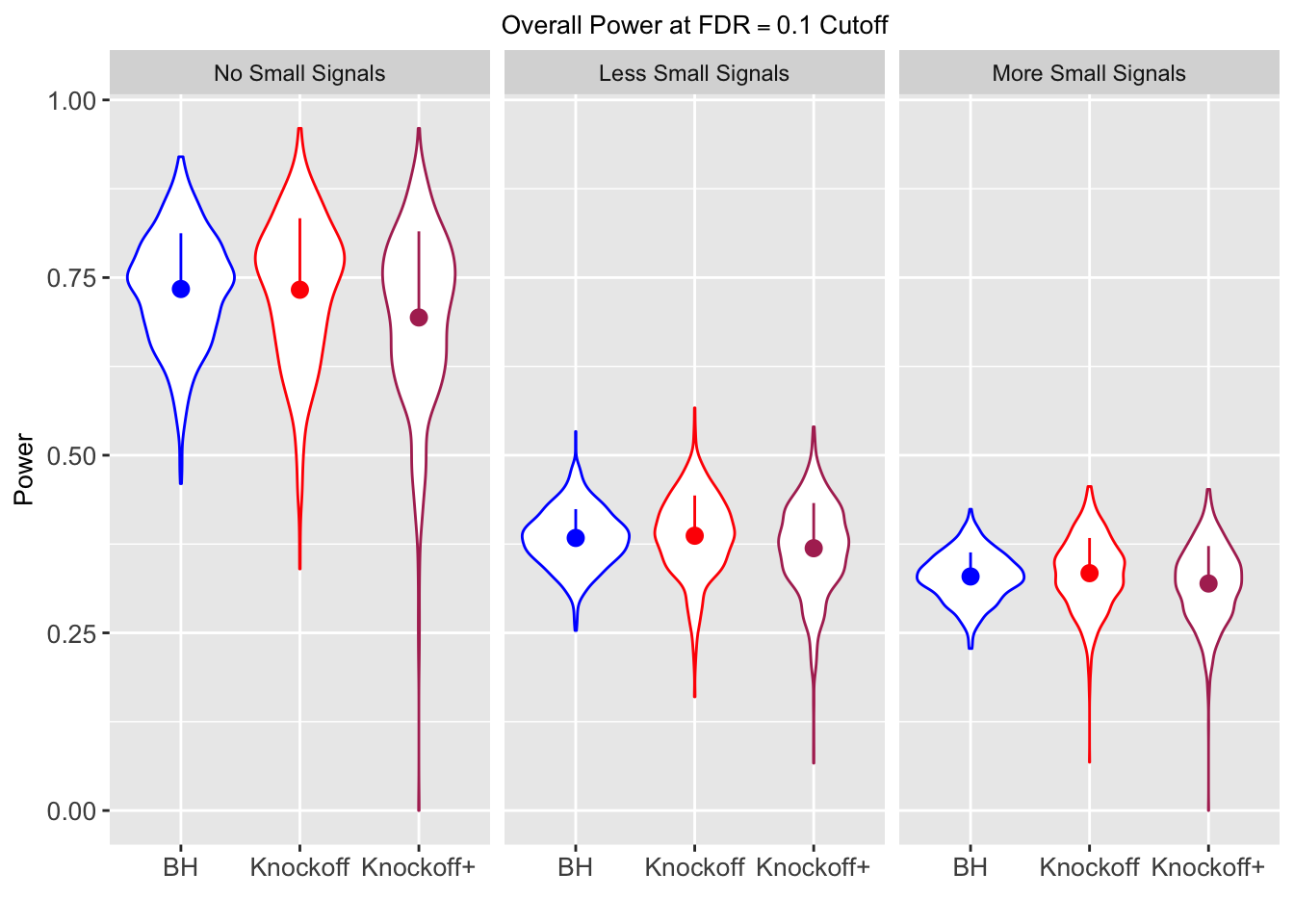
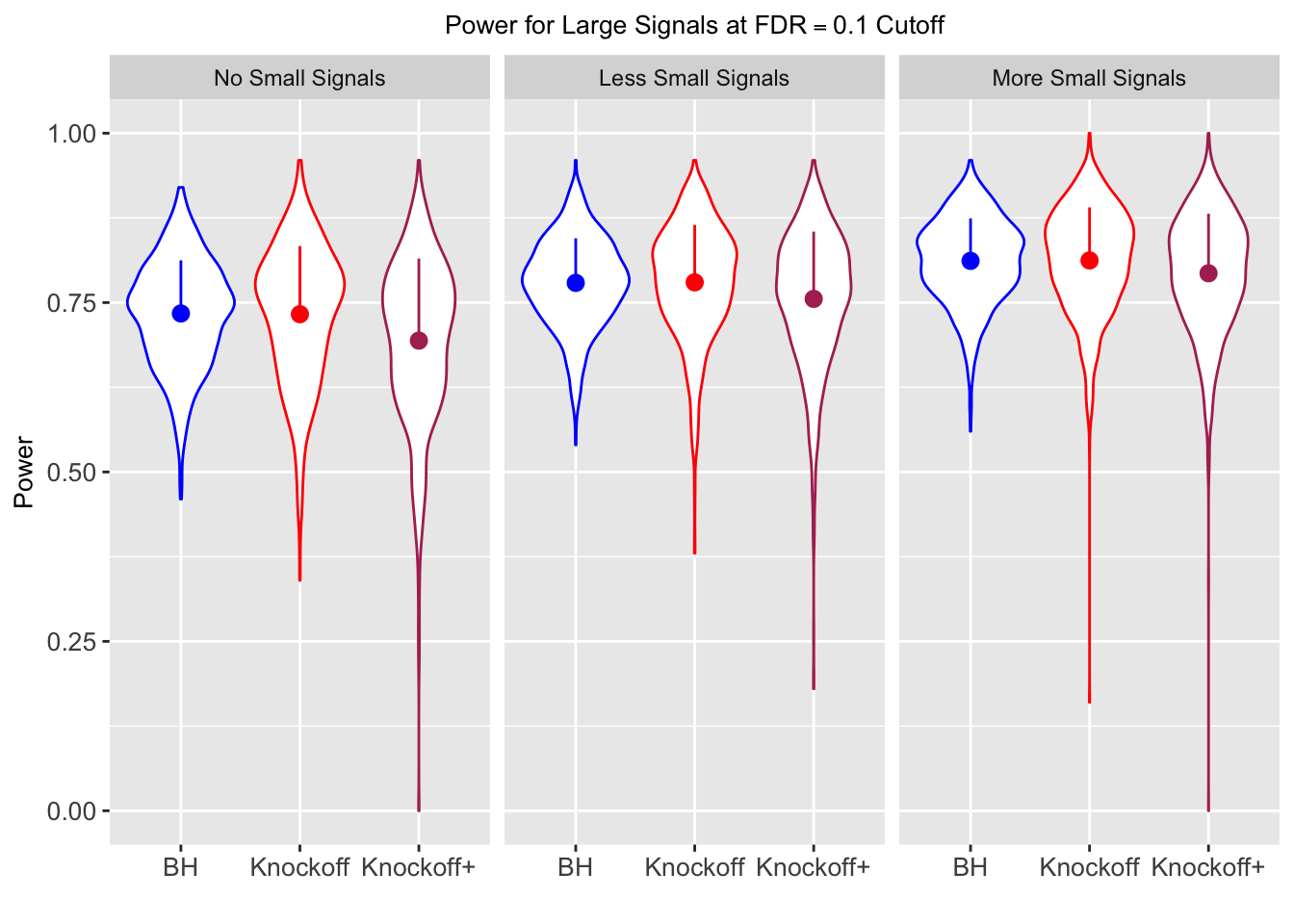
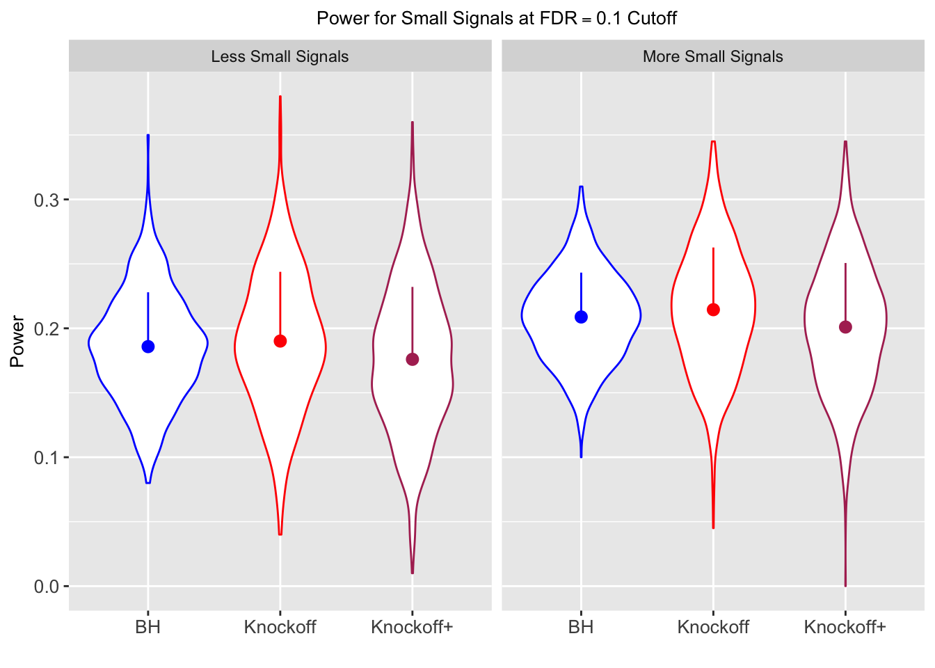
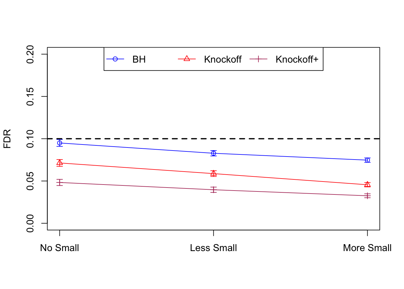
| FDP.BH | FDP.Knockoff | FDP.Knockoff.Plus | Power.BH | Power.Knockoff | Power.Knockoff.Plus | Power.Large.BH | Power.Large.Knockoff | Power.Large.Knockoff.Plus | Power.Small.BH | Power.Small.Knockoff | Power.Small.Knockoff.Plus |
|---|---|---|---|---|---|---|---|---|---|---|---|
| 0.0979 | 0.1082 | 0.0863 | 0.7339 | 0.7329 | 0.6939 | 0.7339 | 0.7329 | 0.6939 | NA | NA | NA |
| 0.0847 | 0.0921 | 0.0795 | 0.3836 | 0.3867 | 0.3691 | 0.7791 | 0.7799 | 0.7555 | 0.1858 | 0.1901 | 0.176 |
| 0.0756 | 0.0817 | 0.0727 | 0.3294 | 0.3340 | 0.3195 | 0.8116 | 0.8122 | 0.7932 | 0.2088 | 0.2145 | 0.201 |
Independent design
\(X_{n \times p}\) has independent columns simulated from \(N(0, 1)\) and then normalized to have \(\|X_j\|_2^2 \equiv 1\).
X <- matrix(rnorm(n * p), n , p)
X <- t(t(X) / sqrt(colSums(X^2)))
Xk <- knockoff::create.fixed(X)
Xk <- Xk$Xk
X <- matrix(rnorm(n * p), n , p)
X <- t(t(X) / sqrt(colSums(X^2)))
Xk <- knockoff::create.fixed(X)
Xk <- Xk$XkX <- matrix(rnorm(n * p), n , p)
X <- t(t(X) / sqrt(colSums(X^2)))
Xk <- knockoff::create.fixed(X)
Xk <- Xk$Xk| FDP.BH | FDP.Knockoff | FDP.Knockoff.Plus | Power.BH | Power.Knockoff | Power.Knockoff.Plus | Power.Large.BH | Power.Large.Knockoff | Power.Large.Knockoff.Plus | Power.Small.BH | Power.Small.Knockoff | Power.Small.Knockoff.Plus |
|---|---|---|---|---|---|---|---|---|---|---|---|
| 0.0950 | 0.0713 | 0.0483 | 0.4344 | 0.5399 | 0.4135 | 0.4344 | 0.5399 | 0.4135 | NA | NA | NA |
| 0.0828 | 0.0587 | 0.0397 | 0.2180 | 0.2106 | 0.1584 | 0.4789 | 0.4820 | 0.3699 | 0.0876 | 0.0749 | 0.0527 |
| 0.0747 | 0.0456 | 0.0325 | 0.1838 | 0.1613 | 0.1243 | 0.5135 | 0.4372 | 0.3432 | 0.1013 | 0.0923 | 0.0696 |
Local correlation design
\(X_{n \times p}\) has correlation \(\Sigma_{ij} = \rho^{|i - j|}\). Each row is independently \(N(0, \Sigma)\) and then normalized to have \(\|X_j\|_2^2 \equiv 1\).
rho <- 0.25
Sigma <- toeplitz(rho^(0 : (p - 1)))
X <- matrix(rnorm(n * p), n , p)
X <- t(t(X) / sqrt(colSums(X^2)))
X <- X %*% chol(Sigma)
Xk <- knockoff::create.fixed(X)
Xk <- Xk$Xk
X <- matrix(rnorm(n * p), n , p)
X <- t(t(X) / sqrt(colSums(X^2)))
X <- X %*% chol(Sigma)
Xk <- knockoff::create.fixed(X)
Xk <- Xk$XkX <- matrix(rnorm(n * p), n , p)
X <- t(t(X) / sqrt(colSums(X^2)))
X <- X %*% chol(Sigma)
Xk <- knockoff::create.fixed(X)
Xk <- Xk$Xk| FDP.BH | FDP.Knockoff | FDP.Knockoff.Plus | Power.BH | Power.Knockoff | Power.Knockoff.Plus | Power.Large.BH | Power.Large.Knockoff | Power.Large.Knockoff.Plus | Power.Small.BH | Power.Small.Knockoff | Power.Small.Knockoff.Plus |
|---|---|---|---|---|---|---|---|---|---|---|---|
| 0.0957 | 0.0563 | 0.0344 | 0.3367 | 0.4985 | 0.3484 | 0.3367 | 0.4985 | 0.3484 | NA | NA | NA |
| 0.0824 | 0.0407 | 0.0249 | 0.1710 | 0.1656 | 0.1070 | 0.3820 | 0.3620 | 0.2348 | 0.0655 | 0.0673 | 0.0431 |
| 0.0738 | 0.0258 | 0.0170 | 0.1441 | 0.1393 | 0.0988 | 0.4137 | 0.4040 | 0.2893 | 0.0767 | 0.0731 | 0.0511 |
Model-\(X\) Knockoffs
Independent design
\(X_{n \times p}\) has independent columns simulated from \(N(0, (1/\sqrt n)^2)\) so they are roughly normalized.
Loaded glmnet 2.0-13| FDP.BH | FDP.Knockoff | FDP.Knockoff.Plus | Power.BH | Power.Knockoff | Power.Knockoff.Plus | Power.Large.BH | Power.Large.Knockoff | Power.Large.Knockoff.Plus | Power.Small.BH | Power.Small.Knockoff | Power.Small.Knockoff.Plus |
|---|---|---|---|---|---|---|---|---|---|---|---|
| 0.0903 | 0.1164 | 0.0935 | 0.4312 | 0.6632 | 0.6124 | 0.4312 | 0.6632 | 0.6124 | NA | NA | NA |
| 0.0782 | 0.1150 | 0.0929 | 0.2213 | 0.3417 | 0.3161 | 0.4808 | 0.6924 | 0.6526 | 0.0916 | 0.1664 | 0.1478 |
| 0.0693 | 0.0923 | 0.0806 | 0.1803 | 0.2731 | 0.2573 | 0.5156 | 0.6962 | 0.6718 | 0.0965 | 0.1674 | 0.1536 |
Local correlation design
\(X_{n \times p}\) has correlation \(\Sigma_{ij} = \rho^{|i - j|}\). Each row is independently \(N(0, \frac1n\Sigma)\).
rho <- 0.5
Sigma <- toeplitz(rho^(0 : (p - 1)))
Sigma.5 <- chol(Sigma)
Cov.X <- Sigma / n| FDP.BH | FDP.Knockoff | FDP.Knockoff.Plus | Power.BH | Power.Knockoff | Power.Knockoff.Plus | Power.Large.BH | Power.Large.Knockoff | Power.Large.Knockoff.Plus | Power.Small.BH | Power.Small.Knockoff | Power.Small.Knockoff.Plus |
|---|---|---|---|---|---|---|---|---|---|---|---|
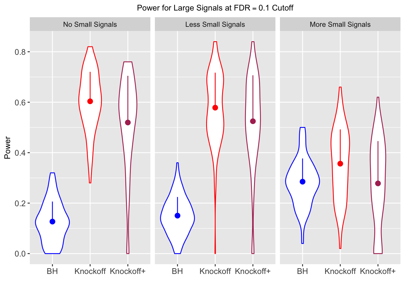
| 0.1199 | 0.1230 | 0.0946 | 0.1268 | 0.6036 | 0.5196 | 0.1268 | 0.6036 | 0.5196 | NA | NA | NA |
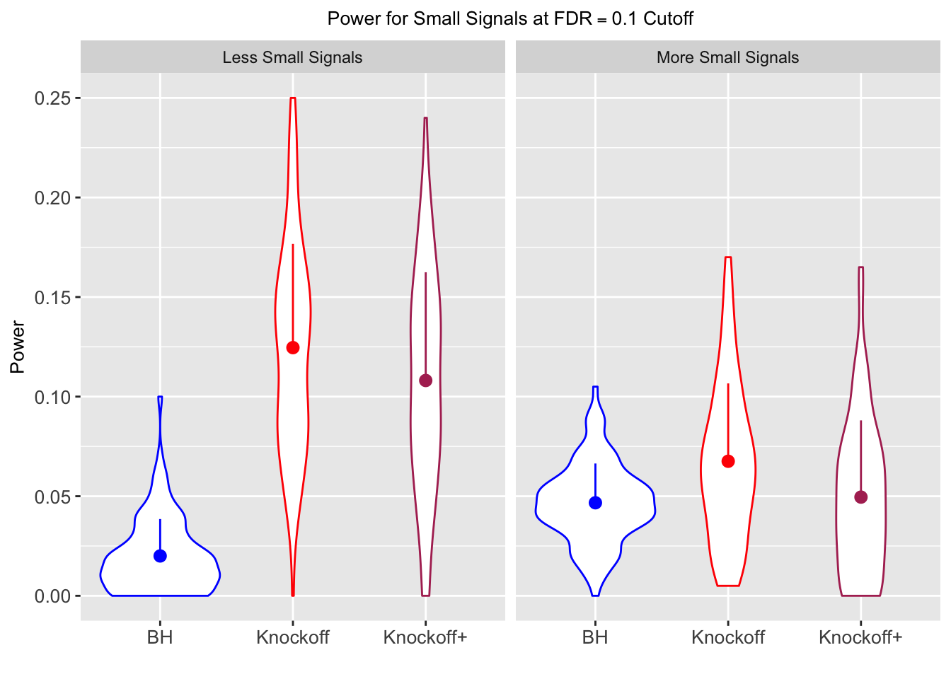
| 0.0840 | 0.0971 | 0.0800 | 0.0635 | 0.2759 | 0.2469 | 0.1504 | 0.5784 | 0.5246 | 0.0200 | 0.1246 | 0.1081 |
| 0.1562 | 0.0671 | 0.0467 | 0.0944 | 0.1253 | 0.0953 | 0.2850 | 0.3564 | 0.2782 | 0.0467 | 0.0676 | 0.0496 |
Session information
sessionInfo()R version 3.4.3 (2017-11-30)
Platform: x86_64-apple-darwin15.6.0 (64-bit)
Running under: macOS High Sierra 10.13.4
Matrix products: default
BLAS: /Library/Frameworks/R.framework/Versions/3.4/Resources/lib/libRblas.0.dylib
LAPACK: /Library/Frameworks/R.framework/Versions/3.4/Resources/lib/libRlapack.dylib
locale:
[1] en_US.UTF-8/en_US.UTF-8/en_US.UTF-8/C/en_US.UTF-8/en_US.UTF-8
attached base packages:
[1] parallel stats graphics grDevices utils datasets methods
[8] base
other attached packages:
[1] knitr_1.20 lattice_0.20-35 doMC_1.3.5 iterators_1.0.9
[5] foreach_1.4.4 ggplot2_2.2.1 reshape2_1.4.3 Matrix_1.2-12
[9] knockoff_0.3.0
loaded via a namespace (and not attached):
[1] Rcpp_0.12.14 magrittr_1.5 munsell_0.4.3 colorspace_1.3-2
[5] rlang_0.1.6 highr_0.6 stringr_1.3.0 plyr_1.8.4
[9] tools_3.4.3 grid_3.4.3 gtable_0.2.0 git2r_0.21.0
[13] htmltools_0.3.6 yaml_2.1.18 lazyeval_0.2.1 rprojroot_1.3-2
[17] digest_0.6.15 tibble_1.4.1 codetools_0.2-15 evaluate_0.10.1
[21] rmarkdown_1.9 labeling_0.3 stringi_1.1.6 pillar_1.0.1
[25] compiler_3.4.3 scales_0.5.0 backports_1.1.2 This R Markdown site was created with workflowr