Introduction

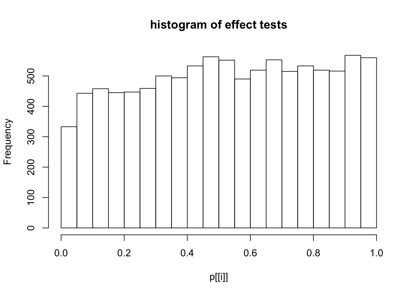
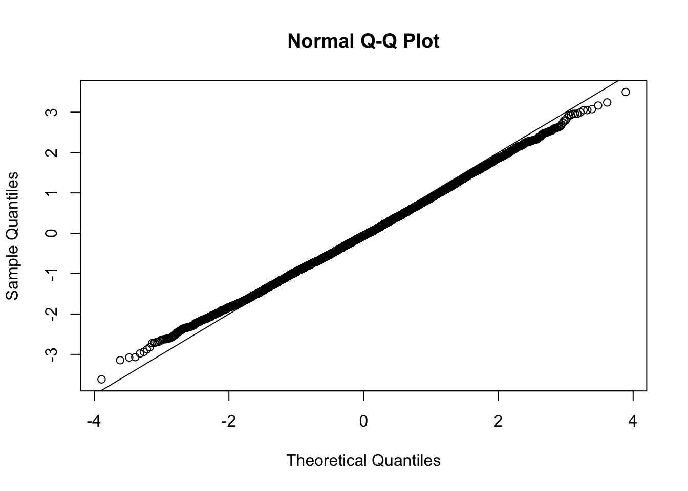
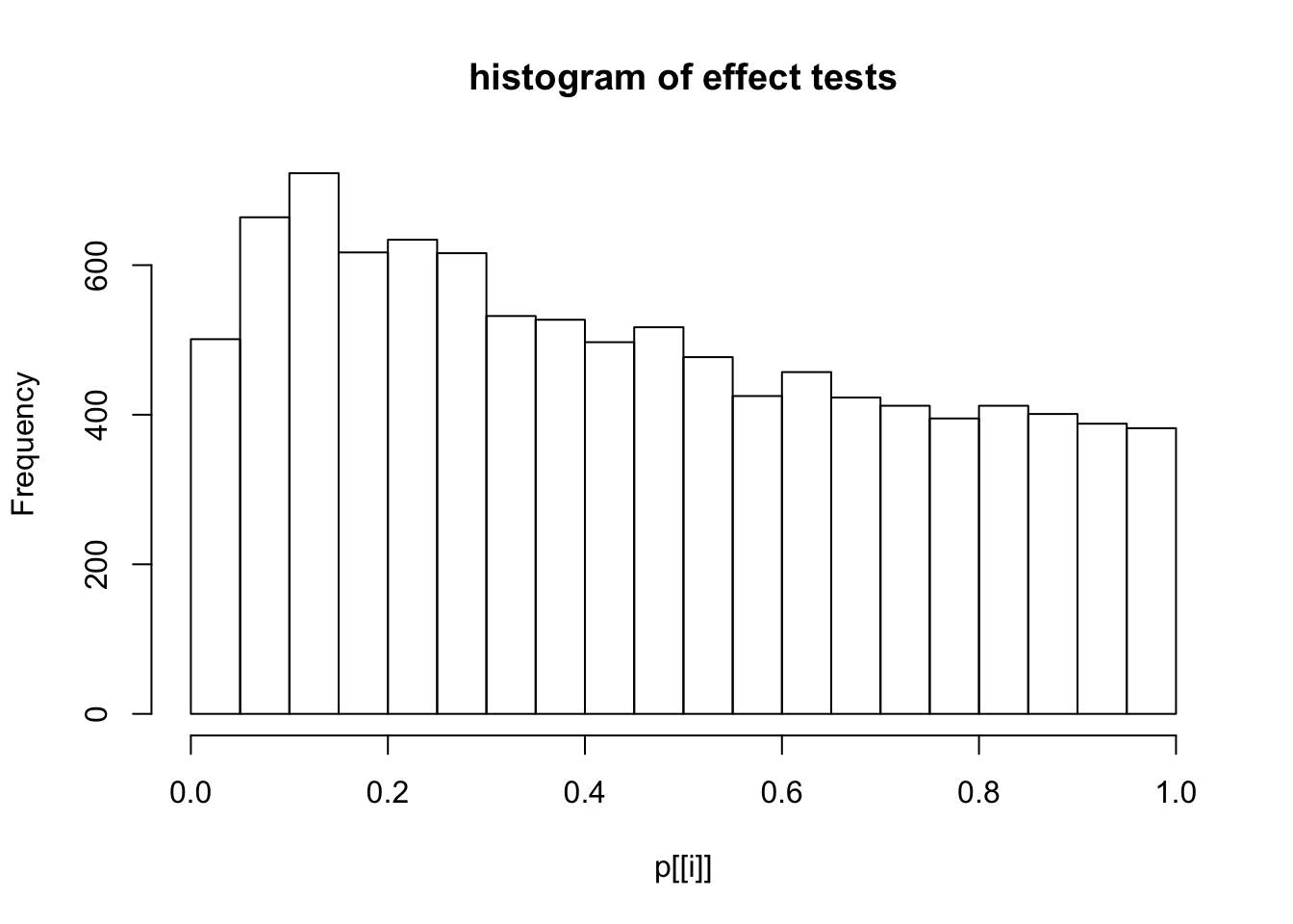
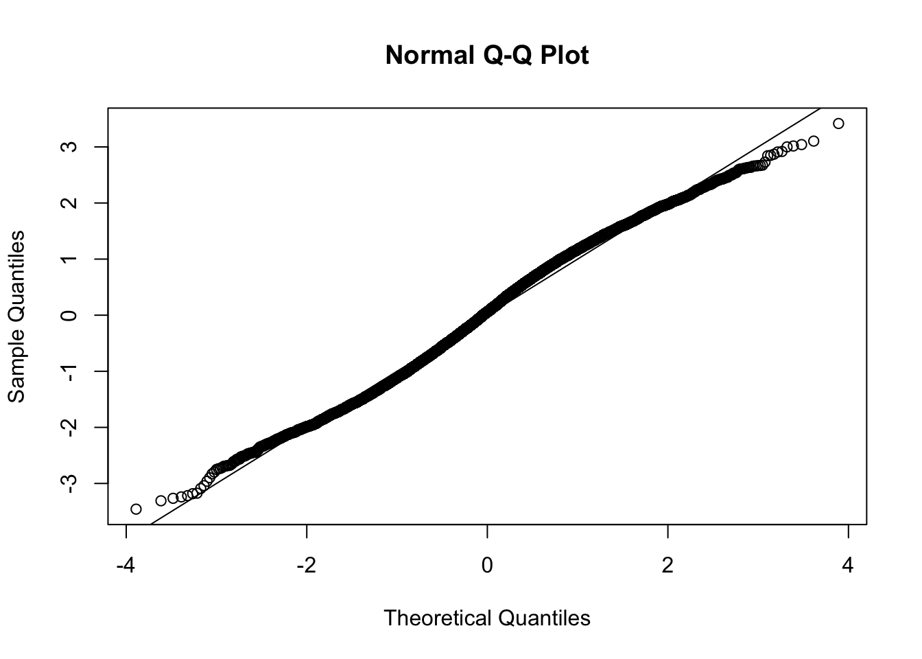
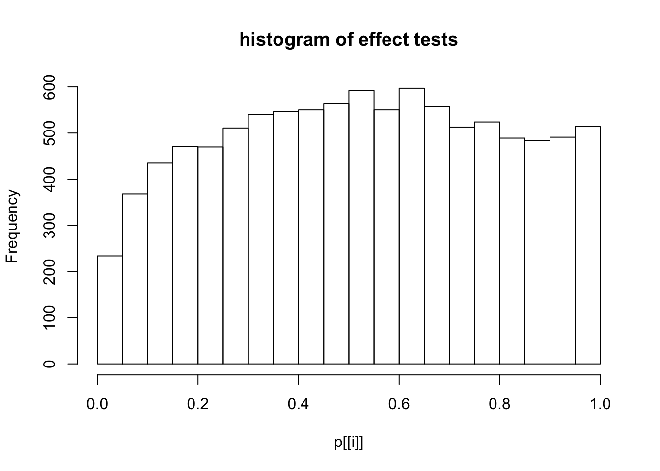
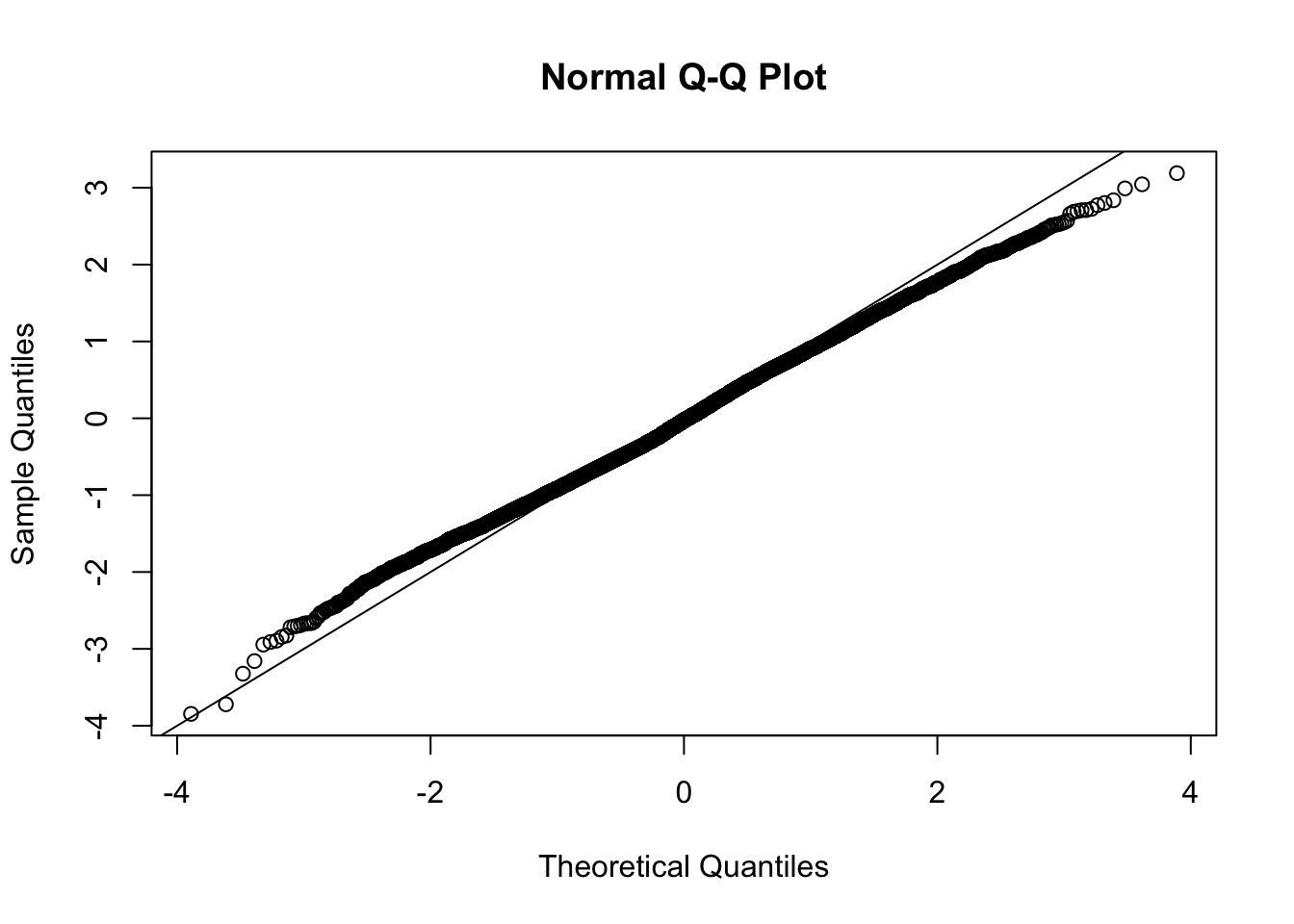
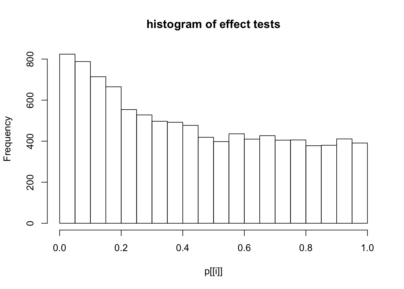
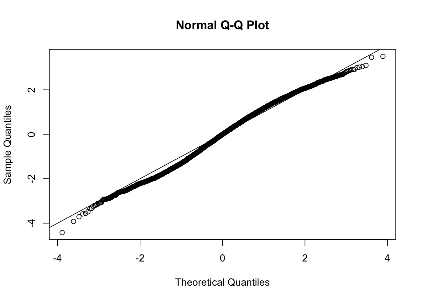
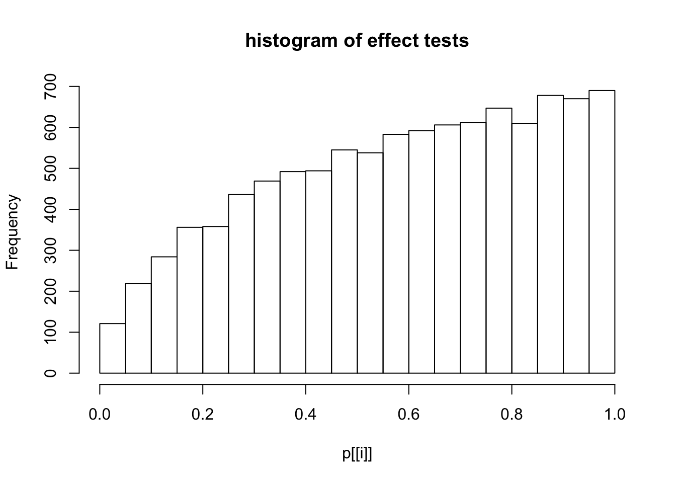
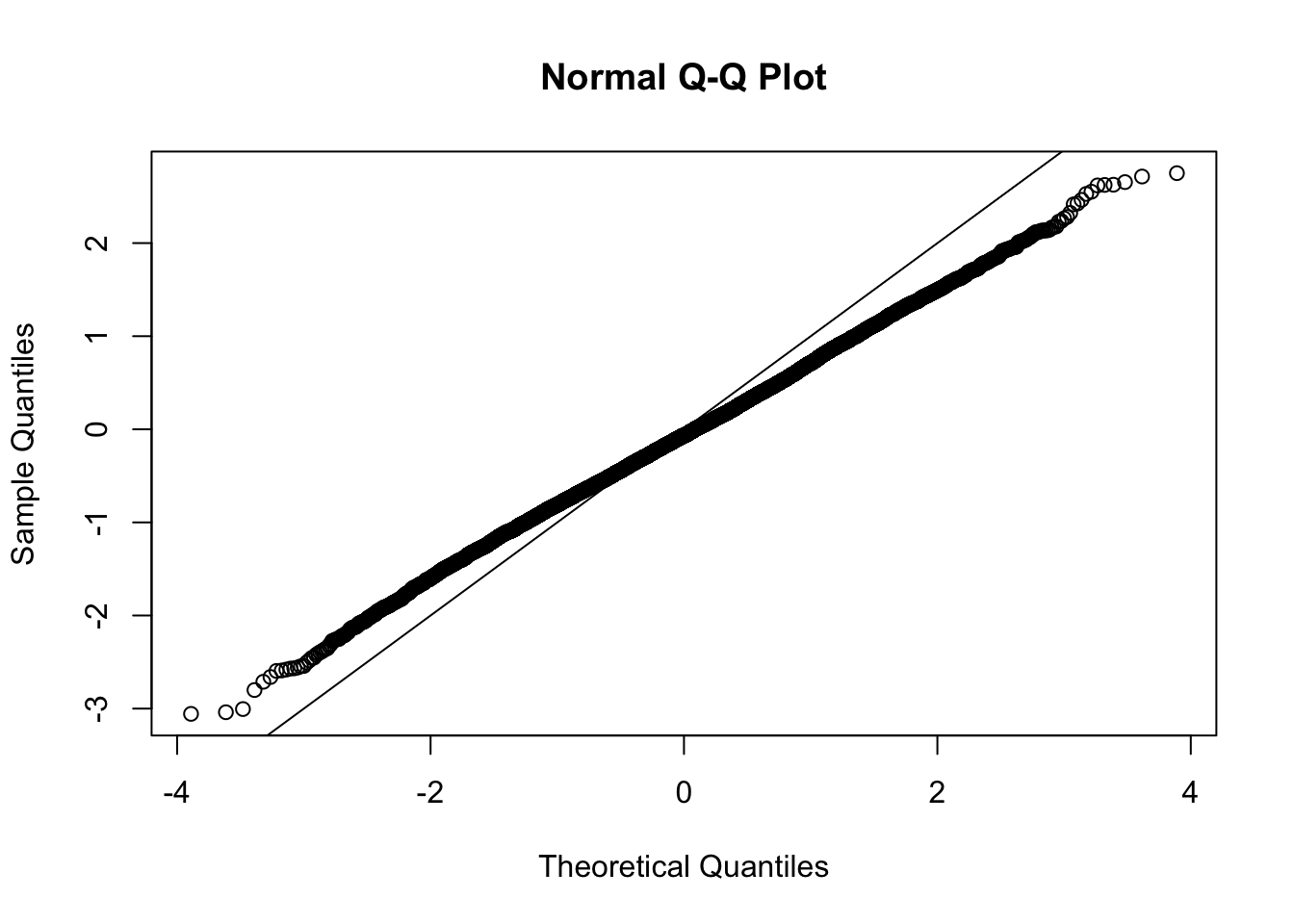
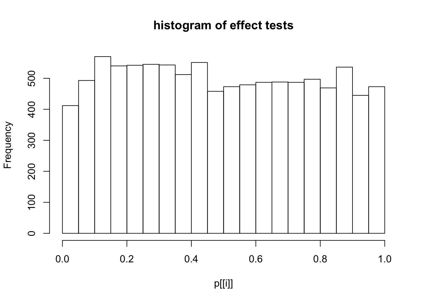
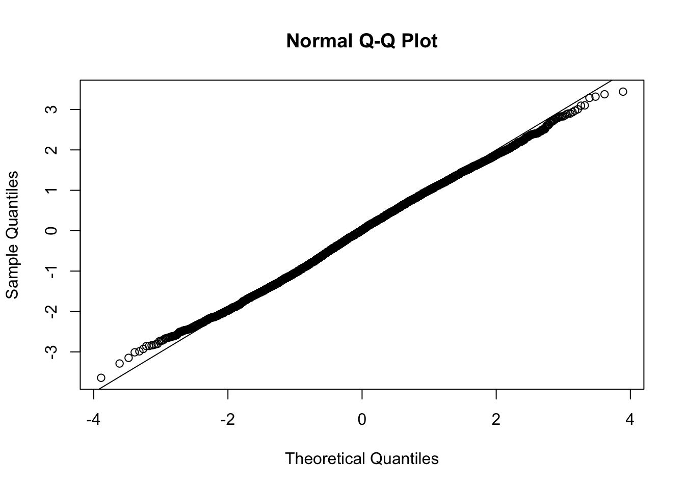
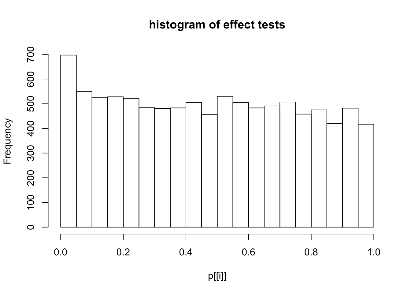
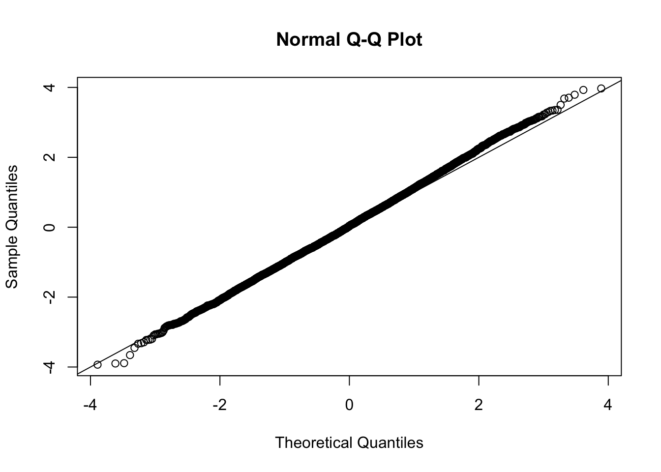
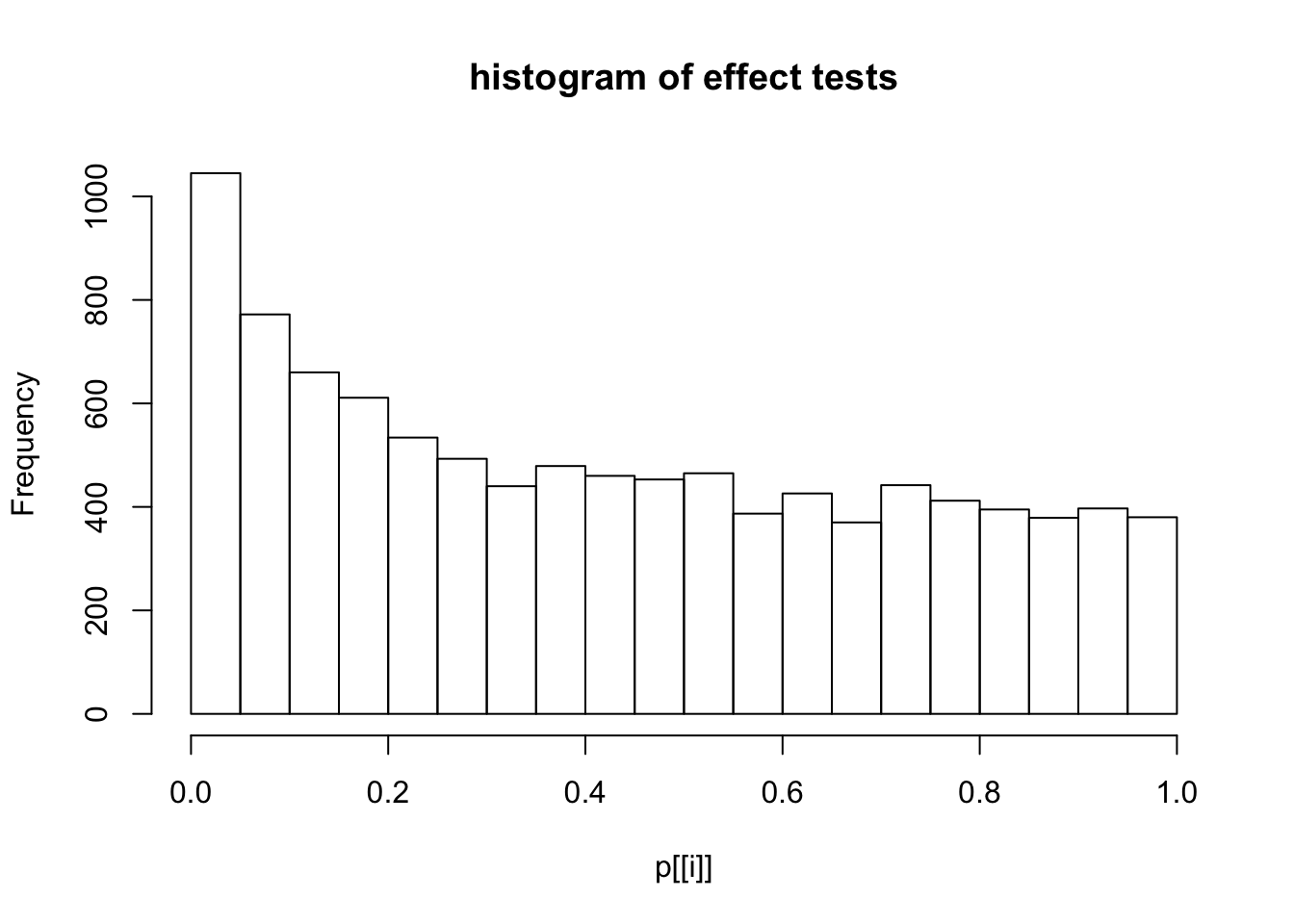
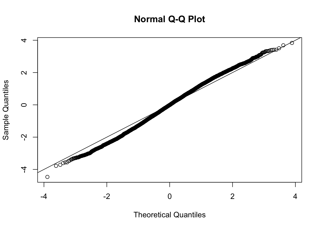
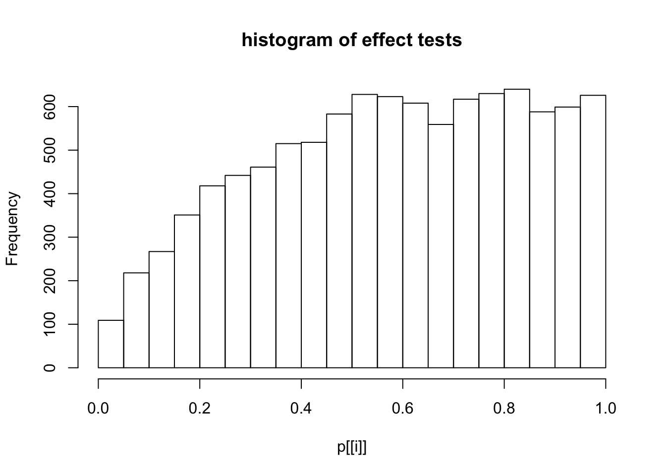
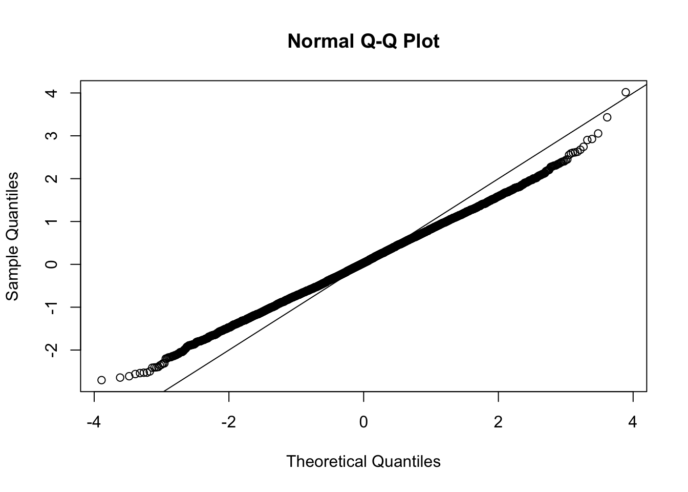
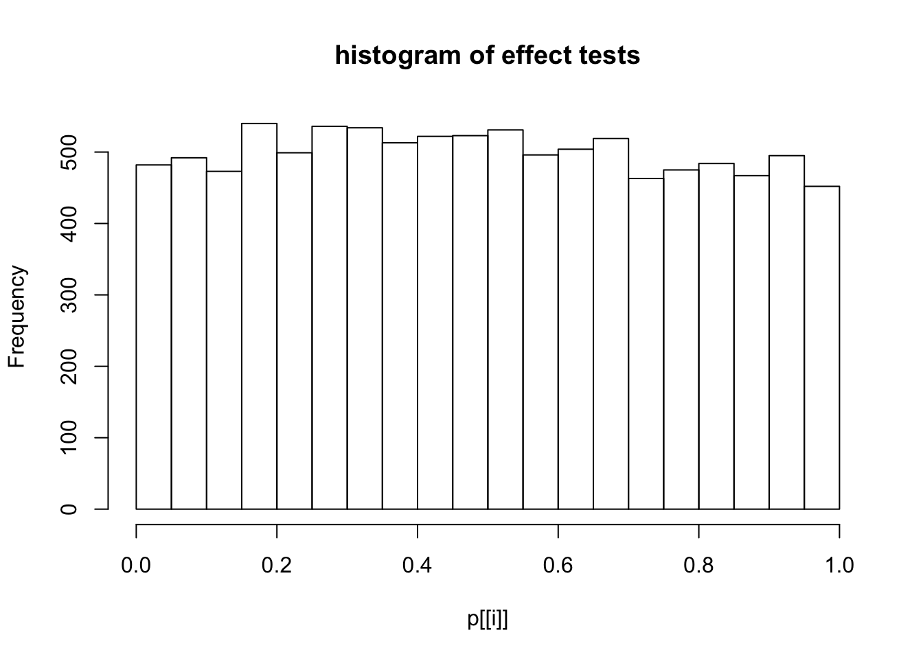
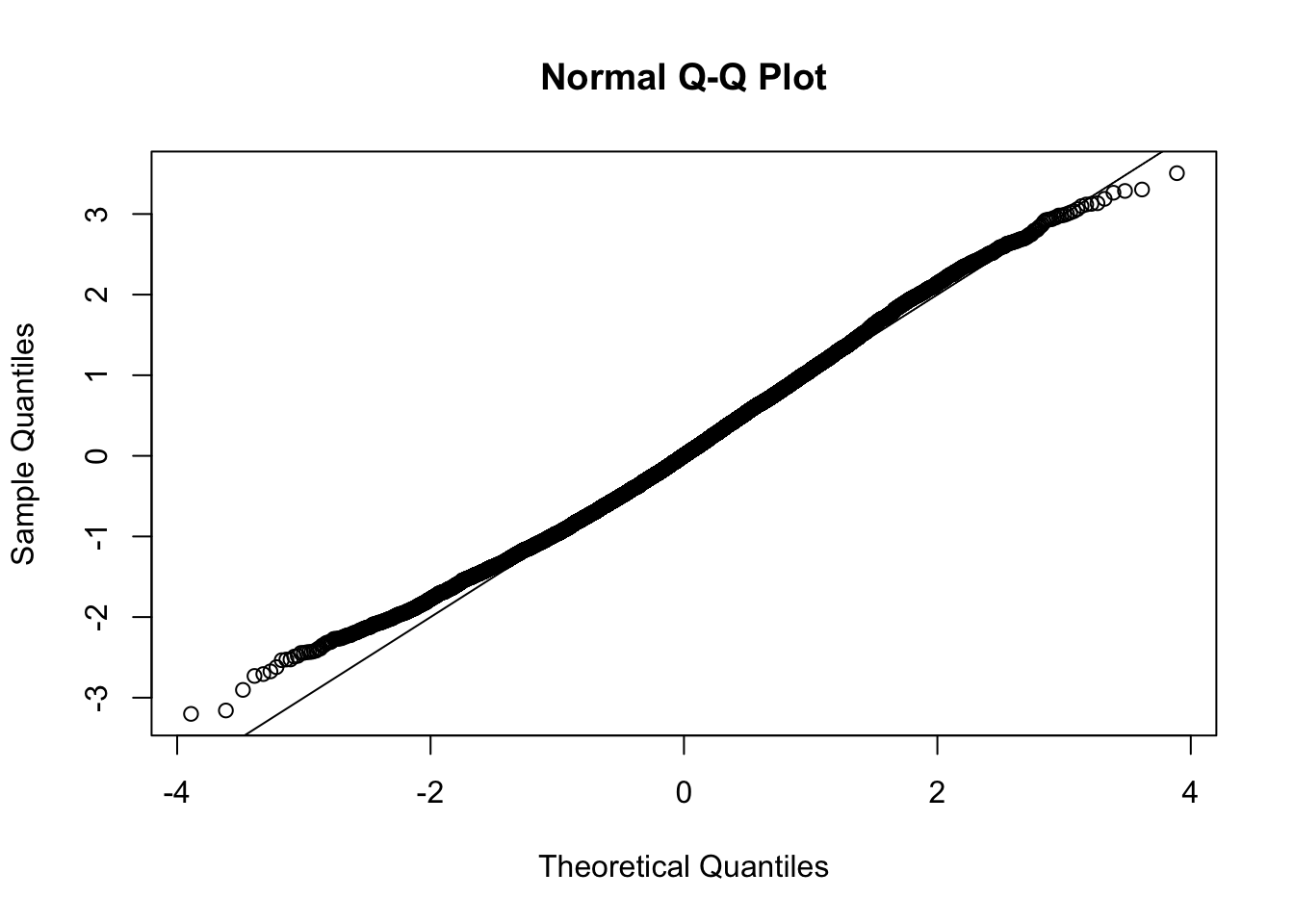
This document simply simulates some null data by randomly sampling two groups of 5 samples from some RNA-seq data (GTEx liver samples). We plot \(p\) value histograms and see the effects of inflation: some distributions are inflated near 0 and others are inflated near 1. However, when we look at the qqplots (here of the z scores, but should be same for p values) we see something that is interesting, although obvious in hindsight: the most extreme p values (z scores) are never “too extreme” (although they are sometimes not extreme enough). The inflation comes from the “not quite so extreme” p values and z scores. This makes sense: when you have positively correlated variables, the most extreme values will tend to be less extreme than when you have independent samples, because you have “effectively” fewer independent samples.

It seems likely this can be exploited to help avoid false positives under positive correlation.

Load in the gtex liver data

library(limma)
library(edgeR)
library(qvalue)
library(ashr)
r = read.csv("../data/Liver.csv")
r = r[,-(1:2)] # remove outliers
#extract top g genes from G by n matrix X of expression
top_genes_index=function(g,X){return(order(rowSums(X),decreasing =TRUE)[1:g])}
lcpm = function(r){R = colSums(r); t(log2(((t(r)+0.5)/(R+1))* 10^6))}
Y=lcpm(r)
subset = top_genes_index(10000,Y)
Y = Y[subset,]
r = r[subset,]

Define voom transform (using code from Mengyin Lu)

voom_transform = function(counts, condition, W=NULL){
  dgecounts = calcNormFactors(DGEList(counts=counts,group=condition))
  #dgecounts = DGEList(counts=counts,group=condition)
  if (is.null(W)){
    design = model.matrix(~condition)
  }else{
    design = model.matrix(~condition+W)
  }
  
  v = voom(dgecounts,design,plot=FALSE)
  lim = lmFit(v)
  betahat.voom = lim$coefficients[,2]
  sebetahat.voom = lim$stdev.unscaled[,2]*lim$sigma
  df.voom = length(condition)-2-!is.null(W)
  
  return(list(v=v,lim=lim,betahat=betahat.voom, sebetahat=sebetahat.voom, df=df.voom, v=v))
}

Make 2 groups of size n, and repeat random sampling.

set.seed(101) 
n = 5 # number in each group
p = list()
z = list()
tscore =list()

for(i in 1:10){
  counts = r[,sample(1:ncol(r),2*n)]
  condition = c(rep(0,n),rep(1,n))
  r.voom = voom_transform(counts,condition)
  r.ebayes = eBayes(r.voom$lim)
  p[[i]] = r.ebayes$p.value[,2]
  tscore[[i]] = r.ebayes$t[,2]
  z[[i]] = sign(r.ebayes$t[,2]) * qnorm(p[[i]]/2)
  hist(p[[i]],main="histogram of effect tests")
  qqnorm(z[[i]])
  abline(a=0,b=1,col=1)
}

sessionInfo()

R version 3.3.2 (2016-10-31)
Platform: x86_64-apple-darwin13.4.0 (64-bit)
Running under: macOS Sierra 10.12.3

locale:
[1] en_US.UTF-8/en_US.UTF-8/en_US.UTF-8/C/en_US.UTF-8/en_US.UTF-8

attached base packages:
[1] stats     graphics  grDevices utils     datasets  methods   base     

other attached packages:
[1] qvalue_2.4.2      edgeR_3.14.0      limma_3.28.5      SQUAREM_2016.10-1
[5] ashr_2.1.2        workflowr_0.3.0   rmarkdown_1.3    

loaded via a namespace (and not attached):
 [1] Rcpp_0.12.9       knitr_1.15.1      magrittr_1.5     
 [4] splines_3.3.2     REBayes_0.62      MASS_7.3-45      
 [7] munsell_0.4.3     doParallel_1.0.10 pscl_1.4.9       
[10] colorspace_1.2-6  lattice_0.20-34   foreach_1.4.3    
[13] plyr_1.8.3        stringr_1.1.0     tools_3.3.2      
[16] parallel_3.3.2    grid_3.3.2        gtable_0.2.0     
[19] git2r_0.18.0      htmltools_0.3.5   iterators_1.0.8  
[22] assertthat_0.1    yaml_2.1.14       rprojroot_1.2    
[25] digest_0.6.11     Matrix_1.2-7.1    reshape2_1.4.1   
[28] ggplot2_2.1.0     codetools_0.2-15  evaluate_0.10    
[31] stringi_1.1.2     scales_0.4.0      Rmosek_7.1.3     
[34] backports_1.0.5   truncnorm_1.0-7