Variance stablizing transformation
Dongyue Xie
Last updated: 2018-10-16
workflowr checks: (Click a bullet for more information)-
✔ R Markdown file: up-to-date
Great! Since the R Markdown file has been committed to the Git repository, you know the exact version of the code that produced these results.
-
✔ Environment: empty
Great job! The global environment was empty. Objects defined in the global environment can affect the analysis in your R Markdown file in unknown ways. For reproduciblity it’s best to always run the code in an empty environment.
-
✔ Seed:
set.seed(20180501)The command
set.seed(20180501)was run prior to running the code in the R Markdown file. Setting a seed ensures that any results that rely on randomness, e.g. subsampling or permutations, are reproducible. -
✔ Session information: recorded
Great job! Recording the operating system, R version, and package versions is critical for reproducibility.
-
Great! You are using Git for version control. Tracking code development and connecting the code version to the results is critical for reproducibility. The version displayed above was the version of the Git repository at the time these results were generated.✔ Repository version: 4c8fd13
Note that you need to be careful to ensure that all relevant files for the analysis have been committed to Git prior to generating the results (you can usewflow_publishorwflow_git_commit). workflowr only checks the R Markdown file, but you know if there are other scripts or data files that it depends on. Below is the status of the Git repository when the results were generated:
Note that any generated files, e.g. HTML, png, CSS, etc., are not included in this status report because it is ok for generated content to have uncommitted changes.Ignored files: Ignored: .DS_Store Ignored: .Rhistory Ignored: .Rproj.user/ Ignored: data/.DS_Store Untracked files: Untracked: analysis/chipexoeg.Rmd Untracked: analysis/talk1011.Rmd Untracked: data/chipexo_examples/ Untracked: data/chipseq_examples/ Untracked: talk.Rmd Untracked: talk.pdf Unstaged changes: Modified: analysis/literature.Rmd Modified: analysis/sigma.Rmd
Expand here to see past versions:
Introduction
Variance stablizing transformation.
\(E(X)=\mu\) and \(Var(X)=g(\mu)\), want to find \(f(\cdot)\) s.t \(Var(f(X))\) has constant variance. Consider the Taylor series expansion of \(f(X)\) around \(\mu\): \(f(X)\approx f(\mu)+(Y-\mu)f'(\mu)\) so we have \([f(X)-f(\mu)]^2\approx (X-\mu)^2(f'(\mu))^2 \Rightarrow Var(f(X))\approx Var(X)(f'(\mu))^2\).
For poisson distribution, \((f'(\mu))^2\propto \mu^{-1}\) so if we take \(Y=\sqrt{X}\) then \(Var(Y)\approx \frac{1}{4}\). This was original proposed by Bartlett in 1936.
For Binomial data, \((f'(\mu))^2\propto 1/(np(1-p))\) so if we take \(Y=sin^{-1}(\sqrt{X/n})\) then \(Var(Y)\approx \frac{1}{2}\).
Anscombe(1948) shows that for \(Y=\sqrt{X+c}\), \(Var(Y)\approx \frac{1}{4}[1+\frac{3-8c}{8\mu}+\frac{32c^2-52c+17}{2\mu^2}]]\). If take \(c=3/8\) and for large \(\mu\), \(Var(Y)\approx 1/4\). Also clearly, \(\lim_{\mu\to 0}Var(\sqrt{X+c})=0\).
mu=c(seq(0,1,length.out = 50),seq(1,10,length.out = 50))
ans=c()
sr=c()
set.seed(12345)
for (i  in 1:100) {
  x=rpois(1e6,mu[i])
  ans[i]=var(sqrt(x+3/8))
  sr[i]=var(sqrt(x))
}
plot(mu,ans,type='l',ylim=c(0,0.5),ylab='')
lines(mu,sr,col=4)
abline(a=0.25,b=0,lty=2)
legend('bottomright',c('anscombe','square root'),lty=c(1,1),col=c(1,4))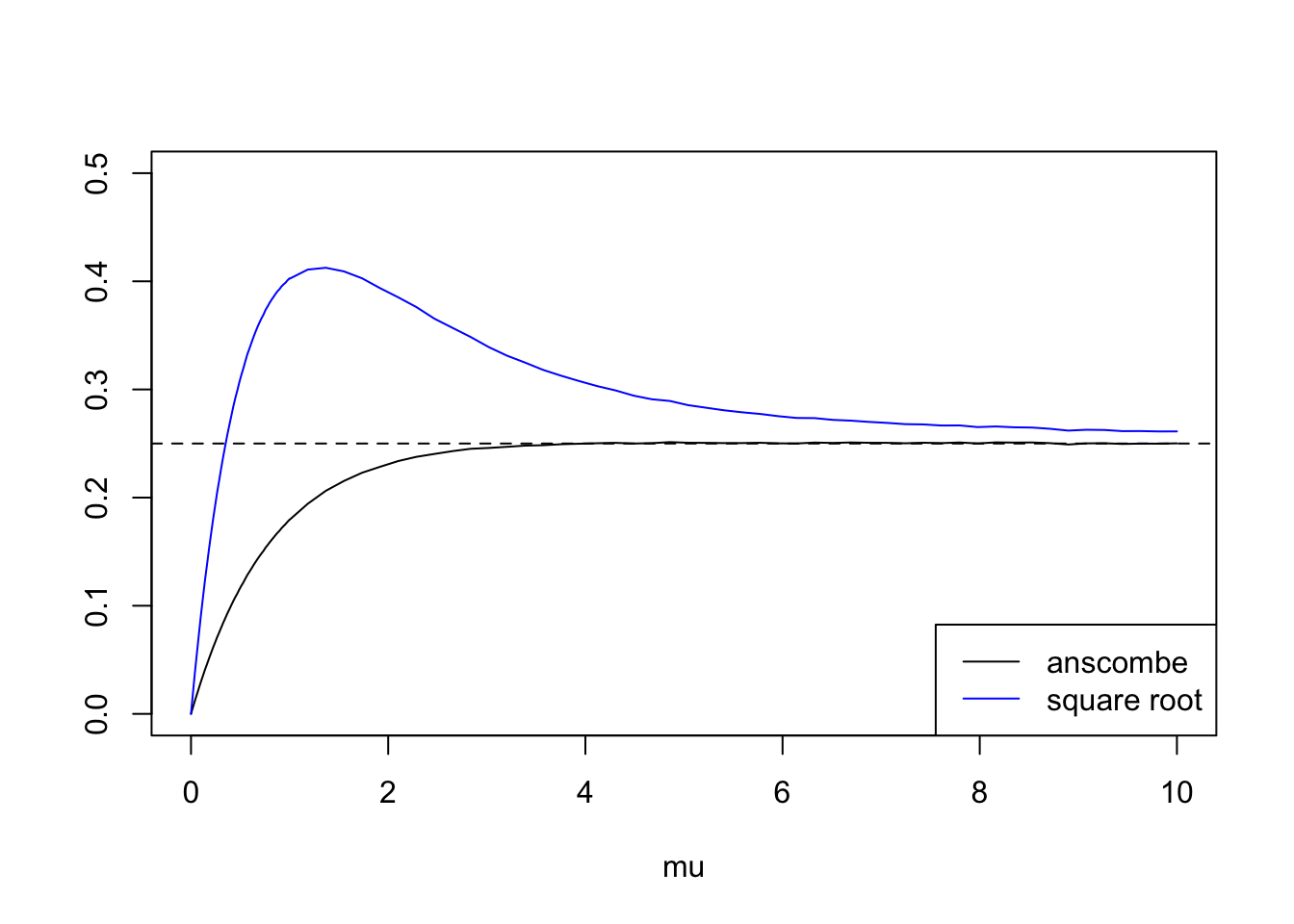
Expand here to see past versions of unnamed-chunk-1-1.png:
| Version | Author | Date |
|---|---|---|
| e24d0a7 | Dongyue Xie | 2018-10-16 |
Compare log and anscombe transformation
Poisson variance stablizing trasformations: square root and Anscombe transformation.
For vst, if we observe \(x=0\), then I use \(var(\sqrt{X+3/8})=0\) instead of \(1/4\).
vst_smooth=function(x,method,ep=1e-5){
  n=length(x)
  if(method=='sr'){
    x.t=sqrt(x)
    x.var=rep(1/4,n)
    x.var[x==0]=0
    mu.hat=(smashr::smash.gaus(x.t,sigma=sqrt(x.var)))^2

  }
  if(method=='anscombe'){
    x.t=sqrt(x+3/8)
    x.var=rep(1/4,n)
    x.var[x==0]=0
    mu.hat=(smashr::smash.gaus(x.t,sigma=sqrt(x.var)))^2-3/8
  }
  if(method=='log'){
    x.t=x
    x.t[x==0]=ep
    x.var=1/x.t
    x.t=log(x.t)
    mu.hat=exp(smashr::smash.gaus(x.t,sigma=sqrt(x.var)))
  }
  return(mu.hat)
}
simu_study=function(m,sig=0,nsimu=100,seed=12345){
set.seed(seed)
sr=c()
an=c()
ashp=c()
for (i in 1:nsimu) {
lambda=exp(log(m)+rnorm(n,0,sig))
x=rpois(n,lambda)
mu.sr=vst_smooth(x,'sr')
mu.an=vst_smooth(x,'anscombe')
mu.ash=smash_gen_lite(x)
sr=rbind(sr,mu.sr)
an=rbind(an,mu.an)
ashp=rbind(ashp,mu.ash)
}
return(list(sr=sr,an=an,ashp=ashp))
}When there are a number of \(0s\) in the observation:
library(ashr)
library(smashrgen)
spike.f = function(x) (0.75 * exp(-500 * (x - 0.23)^2) + 1.5 * exp(-2000 * (x - 0.33)^2) + 3 * exp(-8000 * (x - 0.47)^2) + 2.25 * exp(-16000 *
    (x - 0.69)^2) + 0.5 * exp(-32000 * (x - 0.83)^2))
n = 512
t = 1:n/n
m = spike.f(t)

m=m*2+0.1
range(m)
[1] 0.100000 6.076316result=simu_study(m)
mses=lapply(result, function(x){apply(x, 1, function(y){mean((y-m)^2)})})
plot(m,type='l',main='nugget=0')
lines(result$sr[1,],col=2)
lines(result$an[1,],col=3)
lines(result$ashp[1,],col=4)
legend('topright',c('mean','square root','anscombe','smashgen'),lty=c(1,1,1,1),col=c(1,2,3,4))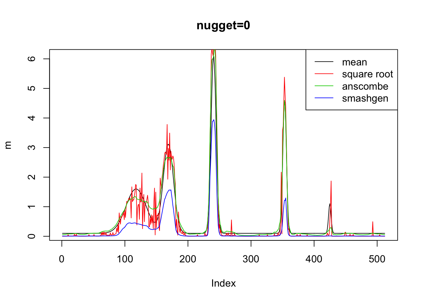
Expand here to see past versions of unnamed-chunk-4-1.png:
| Version | Author | Date |
|---|---|---|
| e24d0a7 | Dongyue Xie | 2018-10-16 |
boxplot(mses,names = c('square root','anscombe','smashgen'),main='nugget=0')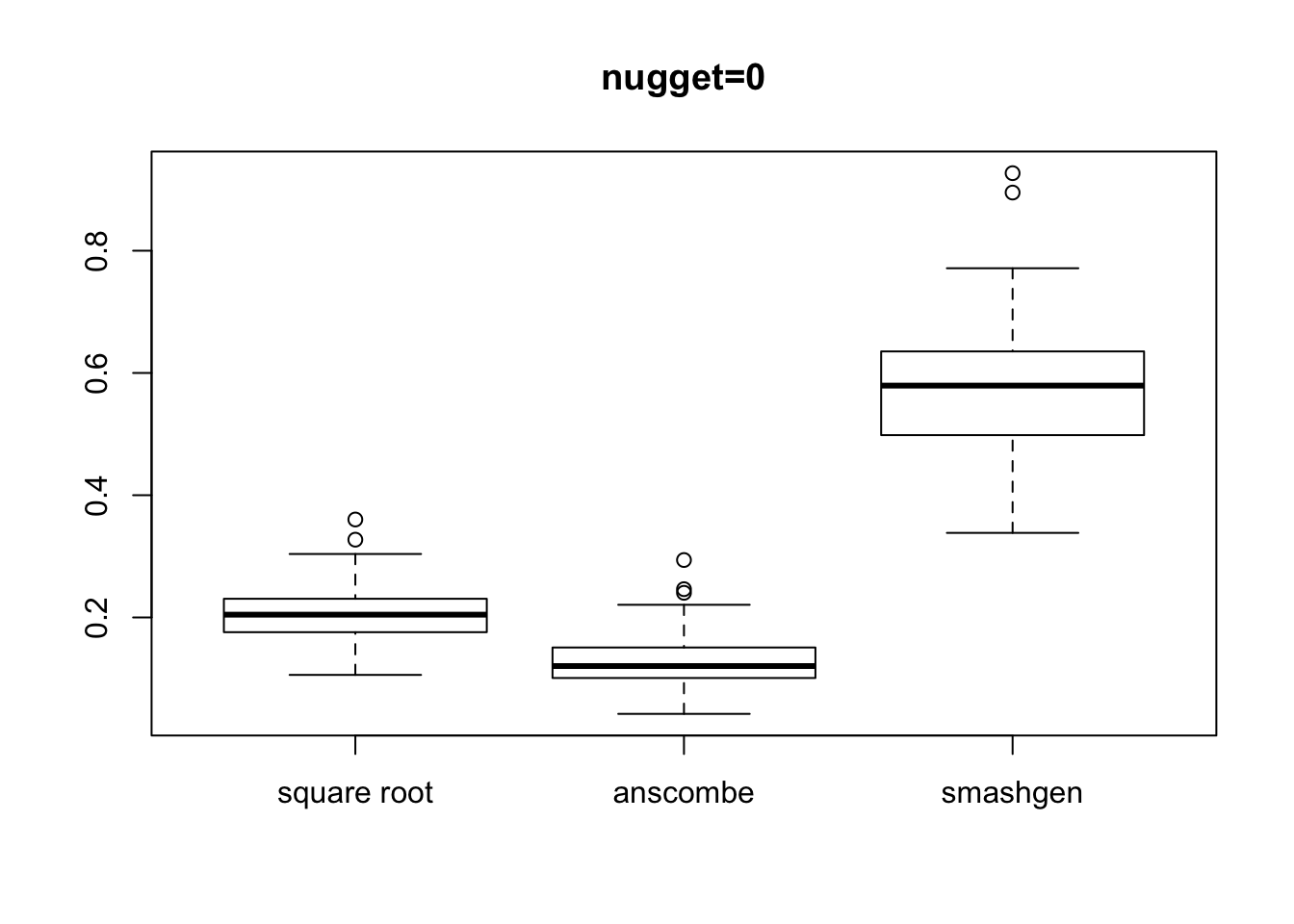
Expand here to see past versions of unnamed-chunk-4-2.png:
| Version | Author | Date |
|---|---|---|
| e24d0a7 | Dongyue Xie | 2018-10-16 |
########
result=simu_study(m,sig=0.5)


mses=lapply(result, function(x){apply(x, 1, function(y){mean((y-m)^2)})})


plot(m,type='l',main='nugget=0.5')
#lines(result$sr[1,],col=2)
lines(result$an[1,],col=3)
lines(result$ashp[1,],col=4)
legend('topright',c('mean','anscombe','smashgen'),lty=c(1,1,1),col=c(1,3,4))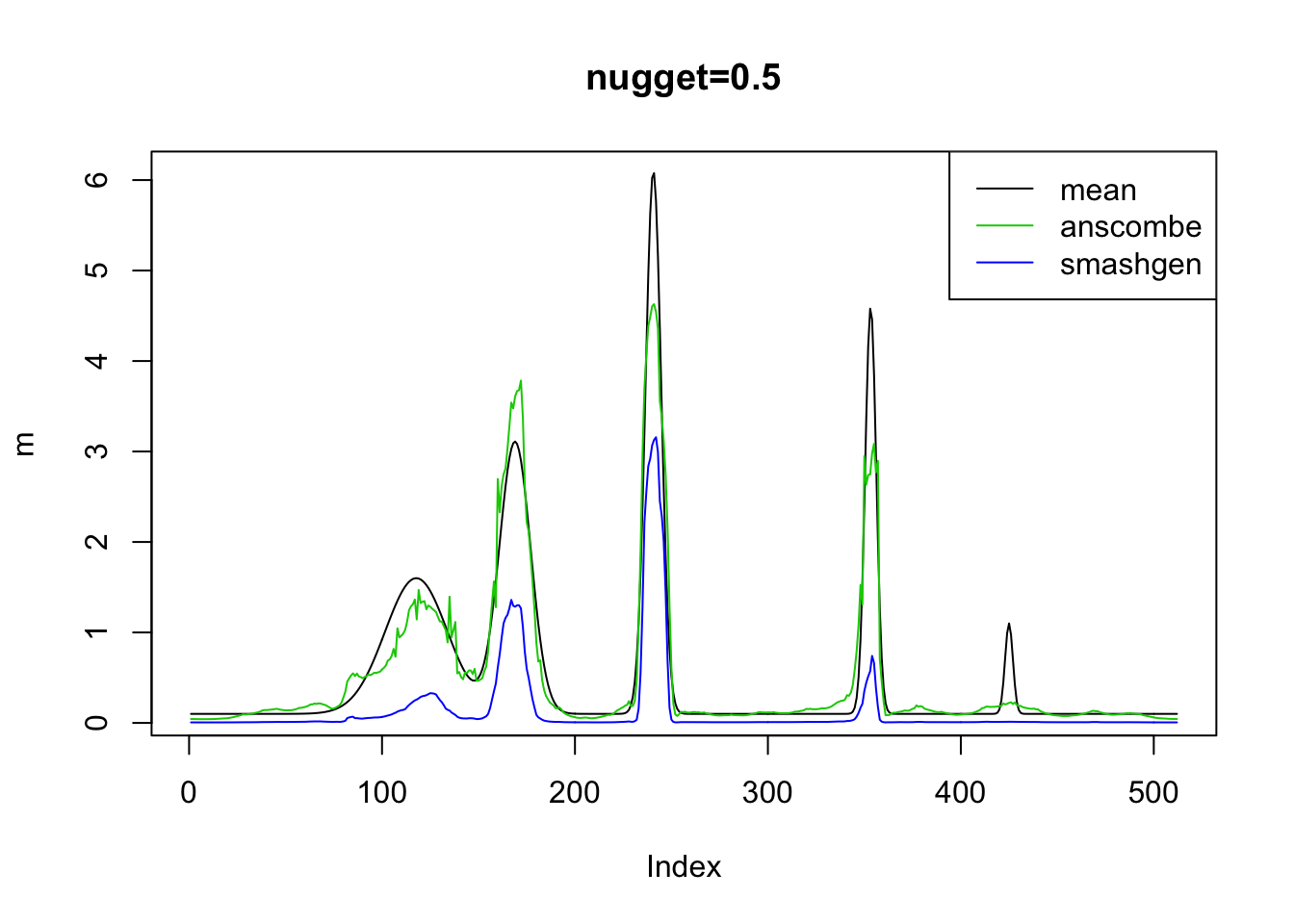
Expand here to see past versions of unnamed-chunk-4-3.png:
| Version | Author | Date |
|---|---|---|
| e24d0a7 | Dongyue Xie | 2018-10-16 |
#legend('topright',c('mean','square root','anscombe','smashgen'),lty=c(1,1,1,1),col=c(1,2,3,4))

boxplot(mses,names = c('square root','anscombe','smashgen'),main='nugget=0.5')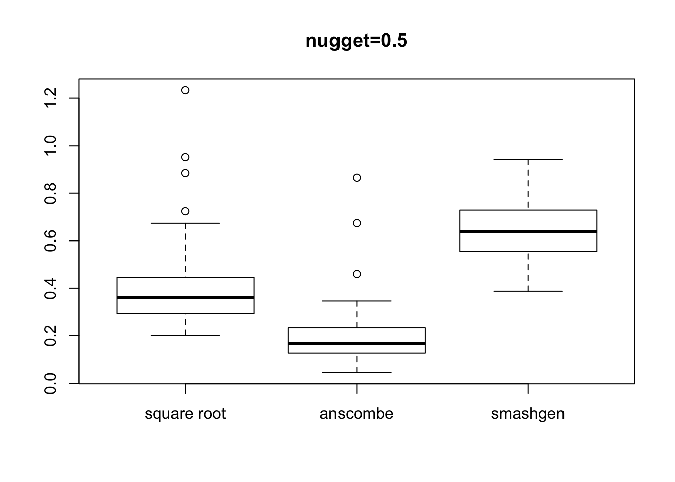
Expand here to see past versions of unnamed-chunk-4-4.png:
| Version | Author | Date |
|---|---|---|
| e24d0a7 | Dongyue Xie | 2018-10-16 |
###############Increase range of mean function:
m=m*20+30
range(m)
[1] 32.0000 151.5263result=simu_study(m)
mses=lapply(result, function(x){apply(x, 1, function(y){mean((y-m)^2)})})
plot(m,type='l',main='nugget=0')
lines(result$sr[1,],col=2)
lines(result$an[1,],col=3)
lines(result$ashp[1,],col=4)
legend('topright',c('mean','square root','anscombe','smashgen'),lty=c(1,1,1,1),col=c(1,2,3,4))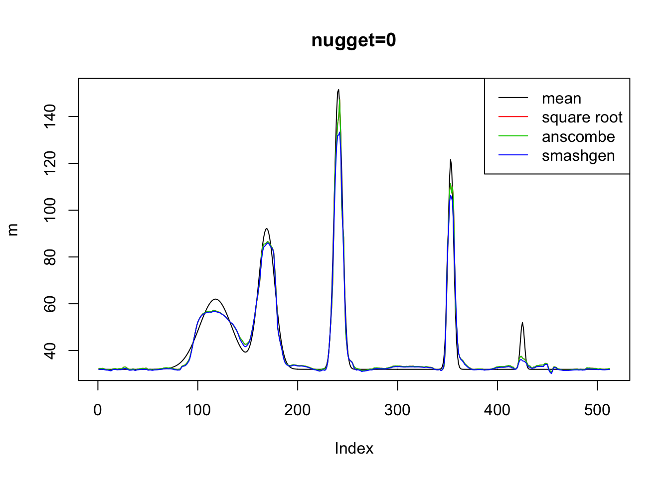
Expand here to see past versions of unnamed-chunk-5-1.png:
| Version | Author | Date |
|---|---|---|
| e24d0a7 | Dongyue Xie | 2018-10-16 |
boxplot(mses,names = c('square root','anscombe','smashgen'),main='nugget=0')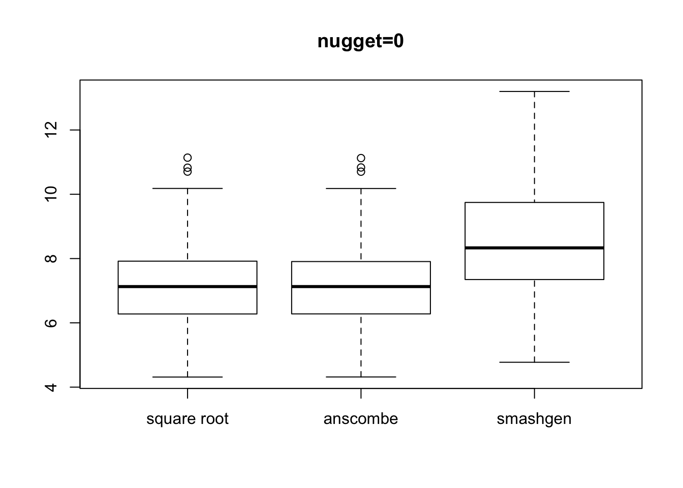
Expand here to see past versions of unnamed-chunk-5-2.png:
| Version | Author | Date |
|---|---|---|
| e24d0a7 | Dongyue Xie | 2018-10-16 |
result=simu_study(m,sig=0.5)

mses=lapply(result, function(x){apply(x, 1, function(y){mean((y-m)^2)})})


plot(m,type='l',main='nugget=0.5')
lines(result$sr[1,],col=2)
lines(result$an[1,],col=3)
lines(result$ashp[1,],col=4)
legend('topright',c('mean','square root','anscombe','smashgen'),lty=c(1,1,1,1),col=c(1,2,3,4))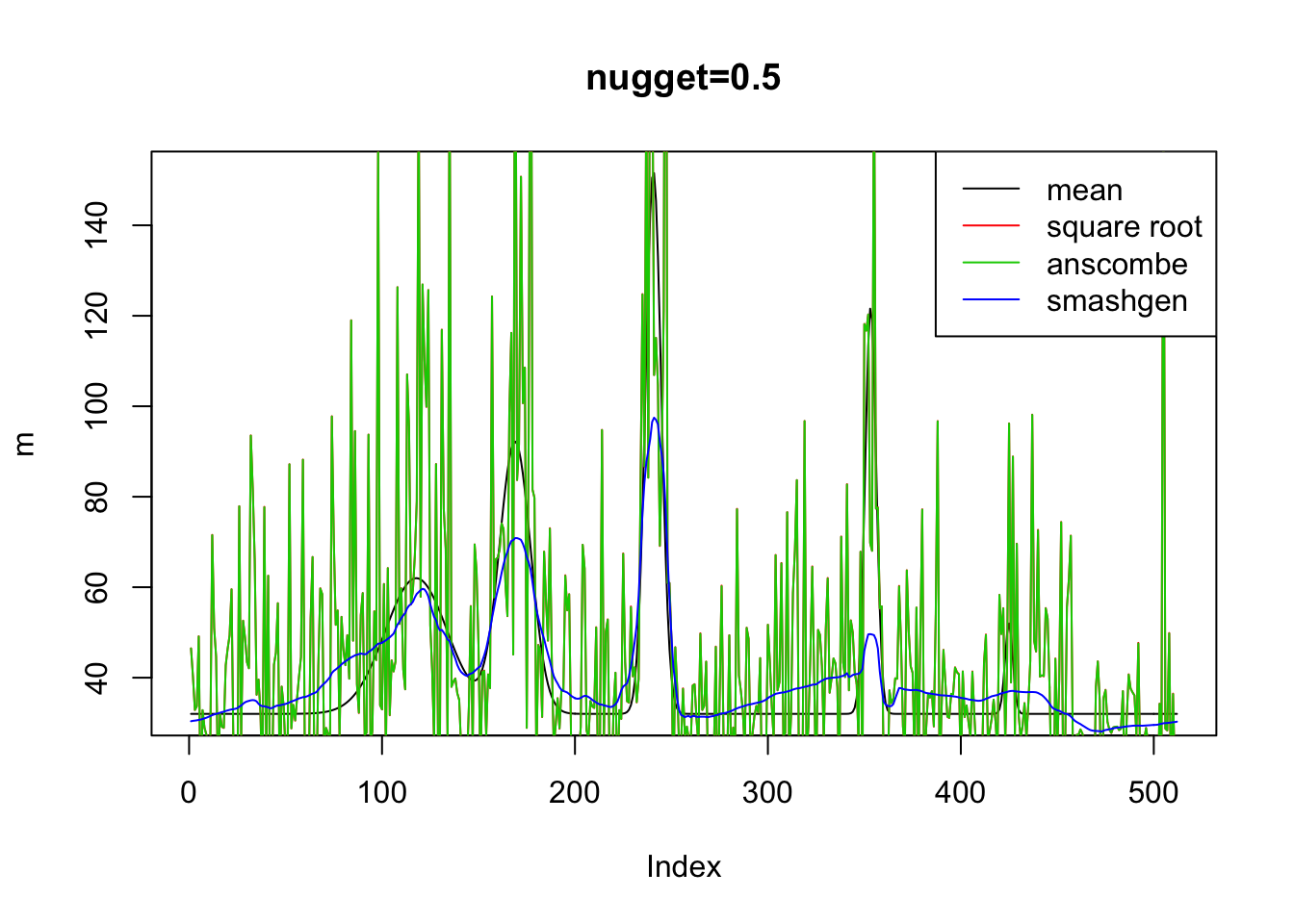
Expand here to see past versions of unnamed-chunk-5-3.png:
| Version | Author | Date |
|---|---|---|
| e24d0a7 | Dongyue Xie | 2018-10-16 |
boxplot(mses,names = c('square root','anscombe','smashgen'),main='nugget=0.5')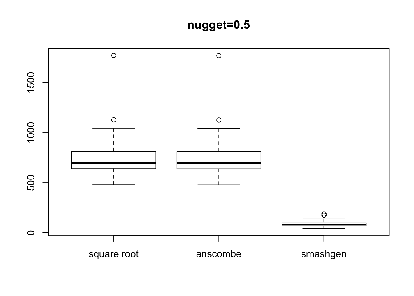
Expand here to see past versions of unnamed-chunk-5-4.png:
| Version | Author | Date |
|---|---|---|
| e24d0a7 | Dongyue Xie | 2018-10-16 |
Session information
sessionInfo()R version 3.5.1 (2018-07-02)
Platform: x86_64-apple-darwin15.6.0 (64-bit)
Running under: macOS High Sierra 10.13.6
Matrix products: default
BLAS: /Library/Frameworks/R.framework/Versions/3.5/Resources/lib/libRblas.0.dylib
LAPACK: /Library/Frameworks/R.framework/Versions/3.5/Resources/lib/libRlapack.dylib
locale:
[1] en_US.UTF-8/en_US.UTF-8/en_US.UTF-8/C/en_US.UTF-8/en_US.UTF-8
attached base packages:
[1] stats graphics grDevices utils datasets methods base
other attached packages:
[1] smashrgen_0.1.0 wavethresh_4.6.8 MASS_7.3-50 caTools_1.17.1.1
[5] smashr_1.2-0 ashr_2.2-7
loaded via a namespace (and not attached):
[1] Rcpp_0.12.18 compiler_3.5.1 git2r_0.23.0
[4] workflowr_1.1.1 R.methodsS3_1.7.1 R.utils_2.7.0
[7] bitops_1.0-6 iterators_1.0.10 tools_3.5.1
[10] digest_0.6.17 evaluate_0.11 lattice_0.20-35
[13] Matrix_1.2-14 foreach_1.4.4 yaml_2.2.0
[16] parallel_3.5.1 stringr_1.3.1 knitr_1.20
[19] REBayes_1.3 rprojroot_1.3-2 grid_3.5.1
[22] data.table_1.11.6 rmarkdown_1.10 magrittr_1.5
[25] whisker_0.3-2 backports_1.1.2 codetools_0.2-15
[28] htmltools_0.3.6 assertthat_0.2.0 stringi_1.2.4
[31] Rmosek_8.0.69 doParallel_1.0.14 pscl_1.5.2
[34] truncnorm_1.0-8 SQUAREM_2017.10-1 R.oo_1.22.0 This reproducible R Markdown analysis was created with workflowr 1.1.1